Predicting the Outcome of NFL Games in the 2024-2025 Season
machine learning
nfl
Follow my attempt to predict the winners and losers of each game in the 2024-2025 NFL season.
Published
September 13, 2024
Code
# Load Librariespacman::p_load("dplyr", # Data Manipulation"nflverse", # NFL Verse Environment"gt", # Nice Tables"tidyr", # Reshaping Data"stringr", # Working with Strings"caret", # Machine Learning"scales", # Percent Formatting"readxl", # Reading Excel Files"writexl", # Writing Excel Filesinstall =FALSE)# Define a Custom Theme - Taken From Andrew Heiss's Blogsblog_theme <-function() {theme_bw() +# Start with theme_bwtheme(panel.grid.minor =element_blank(),plot.background =element_rect(fill ="white", color =NA),plot.title =element_text(face ="bold"),axis.title =element_text(face ="bold"),strip.text =element_text(face ="bold"),strip.background =element_rect(fill ="grey80", color =NA),legend.title =element_text(face ="bold") )}
I am a massive fan of NFL football. I look forward to the inaugural start of the regular season every September and it feels all too soon when the season ends when the Super Bowl is played in February. As much as I love the game-play, the sports shows spinning their narratives, and the social aspect of NFL Sundays, I have been looking for excuses to get my hands on NFL data and having fun with an additional aspect of the game.
Recently, in pursuit of this goal, I went to the Playoff Predictors website, where you can go game-by-game and pick who you think will win each game. It’s a fun exercise that I look forward to every year when the NFL schedule is released and it gives me a picture of what I intuitively think the standings might look like at the conclusion of the upcoming season. Once I got these standings, I played around with the {nflreadr} and {gt} packages to present my predicted standings in a more aesthetically pleasing way.
I like to refer to these as my “vibes-based” predictions because that’s really all they are. However, as a trained social scientist, I am well aware that “vibes” are not wholly informative, well-defined, nor do they contain a great deal of explanatory or predictive power. So, I thought, why not get my hands on more NFL data and try to work up a machine learning based approach? And that is what this blog is for.
Data/Feature Collection
Prior to any fancy modeling, I need to collect some data to predict who wins each game. I want to start off with a major caveat here. I am doing this for fun and educational purposes. Undoubtedly, the predictors I have selected are not reflective of the most advanced analytics nor are they comprehensive. I chose the “lowest hanging fruit” for ease of access. This is probably going to hurt the predictive power of the models (models predict better with more predictive data), but again, humor me!
Overall, I am using the following variables as predictors: whether a team is playing at home, QBR (quarterback rating), passing EPA (expected points added), rushing EPA, receiving EPA, forced fumbles, sacks, interceptions, and passes broken up. Because each prediction is at the game-level, I am using a differenced variable for computational ease (i.e., rather than include the home team’s passing EPA and the away team’s passing EPA in the same model, I just create a difference between the two and use this difference as a predictor for each team). Regardless of which method is used, the predictive performance remained the same after testing.
This selection leaves a lot to be desired. What about more advanced metrics like ELO? What about schematic data (like what type of offense the home team runs v. what type of defense the away team runs, etc.)? What about circumstantial data like whether a key player is out? These are all great things to add that will need to be included in the future! If you’re curious about the data collection syntax, check out the code fold below!
Code
# Load and Clean the QBR Dataqbr <-load_espn_qbr(# Select the 2006-2023 Seasons as Training Dataseasons =2006:2023,# Aggregate at the Week-Levelsummary_type =c("week")) %>%# Exclude Playoff Gamesfilter(season_type =="Regular") %>%# Select Relevant Columnsselect(c(team_abb, season, game_week, qbr_total, pts_added)) %>%# Create Cumulative Averagesgroup_by(season, team_abb) %>%mutate(moving_qbr_mean =cumsum(qbr_total) / game_week,moving_pts_added =cumsum(pts_added / game_week),# Rename Washington for Mergingteam_abb =ifelse(team_abb =="WSH", "WAS", team_abb))# Load and Clean Offensive Stats Dataoffensive <-load_player_stats(# Select the 2006-2023 Seasons as Training Dataseasons =2006:2023,# Filter to Offensestat_type ="offense") %>%# Exclude the Playoffsfilter(season_type =="REG") %>%# Create Team-Level Statsgroup_by(season, recent_team, week) %>%summarise(passing_epa =sum(passing_epa, na.rm =TRUE),rushing_epa =sum(rushing_epa, na.rm =TRUE),receiving_epa =sum(receiving_epa, na.rm =TRUE) ) %>%ungroup() %>%# Create Cumulative Averagesgroup_by(season, recent_team) %>%mutate(moving_passing_epa =cumsum(passing_epa) / week,moving_rushing_epa =cumsum(rushing_epa) / week,moving_receiving_epa =cumsum(receiving_epa) / week) %>%# Keep Relevant Columnsselect(season, recent_team, week, passing_epa, rushing_epa, receiving_epa, moving_passing_epa, moving_rushing_epa, moving_receiving_epa) %>%# Convert Team Abbreviations to a More Standard Form for Mergingmutate(recent_team =ifelse(recent_team =="LA", "LAR", recent_team))# Load and Clean Defensive Stats Datadefensive <-load_player_stats(# Select the 2006-2023 Seasons as Training Dataseasons =2006:2023,# Filter to Defensestat_type ="defense") %>%# Exclude Playoff Gamesfilter(season_type =="REG") %>%# Create Team-Level Statsgroup_by(season, team, week) %>%summarise(tackles =sum(def_tackles, na.rm =TRUE),forced_fumbles =sum(def_fumbles_forced, na.rm =TRUE),sacks =sum(def_sacks, na.rm =TRUE),ints =sum(def_interceptions, na.rm =TRUE),pass_broken =sum( def_pass_defended, na.rm =TRUE) ) %>%ungroup() %>%# Create Cumulative Averagesgroup_by(season, team) %>%mutate(moving_tackles =cumsum(tackles) / week,moving_forced_fumbles =cumsum(forced_fumbles) / week,moving_sacks =cumsum(sacks) / week,moving_ints =cumsum(ints) / week,moving_pass_broken =cumsum(pass_broken) / week) %>%# Keep Relevant Columnsselect(season, team, week, tackles, forced_fumbles, sacks, ints, pass_broken, moving_tackles, moving_forced_fumbles, moving_sacks, moving_ints, moving_pass_broken) %>%# Convert Team Abbreviations to a More Standard Form for Mergingmutate(team =ifelse(team =="LA", "LAR", team))# Load and Clean Schedules Dataseasons <-load_schedules(seasons =2006:2023)# Convert the Data From Dyadic to Monadicseasons <-clean_homeaway(seasons) %>%# Exclude Playoff Gamesfilter(game_type =="REG") %>%# Create a Home Team Variablemutate(home =ifelse(location =="home", 1, 0),# Create a Win Variablewin =ifelse(team_score > opponent_score, 1, 0)) %>%# Keep Relevant Columnsselect(game_id, season, week, team, opponent, home, win) %>%# Convert Team Abbreviations to a More Standard Form for Mergingmutate(team =ifelse(team =="LA", "LAR", team),opponent =ifelse(opponent =="LA", "LAR", opponent))# Merge This Datamerged <-inner_join(seasons, qbr, by =c("season", "team"="team_abb", "week"="game_week")) %>%inner_join(offensive, by =c("season", "team"="recent_team", "week")) %>%inner_join(defensive, by =c("season", "team", "week"))merged <- merged %>%group_by(game_id) %>%# Create Opponent Columns# This Work Because Each Team Opponent Is In a Paired Set of Rows# The Opponent Is Always the Second Observation# Basically, This Just Reverses Cumulative Stats For Each Team Under a Different Namemutate(opp_qbr =lead(moving_qbr_mean),opp_qbr =ifelse(is.na(opp_qbr), lag(moving_qbr_mean), opp_qbr),opp_pass_epa =lead(moving_passing_epa),opp_pass_epa =ifelse(is.na(opp_pass_epa), lag(moving_passing_epa), opp_pass_epa),opp_rushing_epa =lead(moving_rushing_epa),opp_rushing_epa =ifelse(is.na(opp_rushing_epa), lag(moving_rushing_epa), opp_rushing_epa),opp_receiving_epa =lead(moving_receiving_epa),opp_receiving_epa =ifelse(is.na(opp_receiving_epa), lag(moving_receiving_epa), opp_receiving_epa),opp_tackles =lead(moving_tackles),opp_tackles =ifelse(is.na(opp_tackles), lag(moving_tackles), opp_tackles),opp_forced_fumbles =lead(moving_forced_fumbles),opp_forced_fumbles =ifelse(is.na(opp_forced_fumbles), lag(moving_forced_fumbles), opp_forced_fumbles),opp_sacks =lead(moving_sacks),opp_sacks =ifelse(is.na(opp_sacks), lag(moving_sacks), opp_sacks),opp_ints =lead(moving_ints),opp_ints =ifelse(is.na(opp_ints), lag(moving_ints), opp_ints),opp_pass_broken =lead(moving_pass_broken),opp_pass_broken =ifelse(is.na(opp_pass_broken), lag(moving_pass_broken), opp_pass_broken) ) %>%# Create Differenced Columnsmutate(qbr_diff = moving_qbr_mean - opp_qbr,pass_epa_diff = moving_passing_epa - opp_pass_epa,rushing_epa_diff = moving_rushing_epa - opp_rushing_epa,receiving_epa_diff = moving_receiving_epa - opp_receiving_epa,tackles_diff = moving_tackles - opp_tackles,forced_fumbles_diff = moving_forced_fumbles - opp_forced_fumbles,sacks_diff = moving_sacks - opp_sacks,ints_diff = moving_ints - opp_ints,pass_broken_diff = moving_pass_broken - opp_pass_broken ) %>%# Make the Outcome Column Suitable for Classificationmutate(win =factor(win, levels =c(0, 1), labels =c("Lose", "Win"))) %>%# Drop NAs Because They Will Create Problemsdrop_na()
Machine Learning Algorithms Limitations
Okay, now onto the actual machine learning algorithms that will be used. Again, nothing super fancy here. In the interest of keeping things simple at first, I chose to just explore how predictive accuracy fluctuates between four popular ML algorithms (logistic regression… which makes me cringe to refer to it as “ML”, random forest, support vector machine (SVM), and XGBoost). For those curious, I did engage in hyper-parameter tuning, but, no amount of tuning really improved the model results that much, and I felt that, in the interest of simplicity and computational time, it would be best to just include four basic ML algorithms for now.
# For Reproducibilityset.seed(1234)# Establish a Cross-Validation Methodcv_method <-trainControl(method ="cv",number =10,classProbs =TRUE,summaryFunction = twoClassSummary)# Fit Models# Logistic Regressionlog_fit <-train(win ~ home + qbr_diff + pass_epa_diff + rushing_epa_diff + receiving_epa_diff + forced_fumbles_diff + sacks_diff + ints_diff + pass_broken_diff, data = merged,method ="glm",family ="binomial",trControl = cv_method,metric ="ROC")# Save Model Results So I Don't Have to Re-Train Every TimesaveRDS(log_fit, "data-and-analysis/log_fit_model.rds")# Random Forestrf_fit <-train(win ~ home + qbr_diff + pass_epa_diff + rushing_epa_diff + receiving_epa_diff + forced_fumbles_diff + sacks_diff + ints_diff + pass_broken_diff, data = merged,method ="rf",trControl = cv_method,metric ="ROC")saveRDS(rf_fit, "data-and-analysis/rf_fit_model.rds")# Support Vector Machinesv_fit <-train(win ~ home + qbr_diff + pass_epa_diff + rushing_epa_diff + receiving_epa_diff + forced_fumbles_diff + sacks_diff + ints_diff + pass_broken_diff, data = merged,method ="svmLinear",trControl = cv_method,metric ="ROC")saveRDS(sv_fit, "data-and-analysis/sv_fit_model.rds")# XGBoostxgb_fit <-train(win ~ qbr_diff + pass_epa_diff + rushing_epa_diff + receiving_epa_diff + forced_fumbles_diff + sacks_diff + ints_diff + pass_broken_diff, data = merged,method ="xgbTree",trControl = cv_method,metric ="ROC")saveRDS(xgb_fit, "data-and-analysis/xgb_fit_model.rds")# Store the Predictive Accuracy Results in a Tableresults <-tibble(Model =c("Logistic Regression", "Random Forest", "SVM", "XGBoost"),# Store ROC MetricsROC =c(# which.max() Doesn't Do Anything Here, But It Would If I Had Tons of Different# Models for Each Model Type. It Would Select the Model with the Highest Predictive# Power. Not Helpful Here Since I Am Only Running One Model of Each Type, But It's# A Useful Reference That I Want to Keep for the Future log_fit$results[which.max(log_fit$results$ROC), "ROC"], rf_fit$results[which.max(rf_fit$results$ROC), "ROC"], sv_fit$results[which.max(sv_fit$results$ROC), "ROC"], xgb_fit$results[which.max(xgb_fit$results$ROC), "ROC"] ),# Store Accurate Predictions PercentageAccuracy =c( (log_fit$results$Spec[which.max(log_fit$results$ROC)] + log_fit$results$Sens[which.max(log_fit$results$ROC)]) /2, (rf_fit$results$Spec[which.max(rf_fit$results$ROC)] + rf_fit$results$Sens[which.max(rf_fit$results$ROC)]) /2, (sv_fit$results$Spec[which.max(sv_fit$results$ROC)] + sv_fit$results$Sens[which.max(sv_fit$results$ROC)]) /2, (xgb_fit$results$Spec[which.max(xgb_fit$results$ROC)] + xgb_fit$results$Sens[which.max(xgb_fit$results$ROC)]) /2 ))
Model Evaluation
So, how did these models fair? Eh… not great, as you can see below
results
# A tibble: 4 × 3
  Model                 ROC Accuracy
  <chr>               <dbl>    <dbl>
1 Logistic Regression 0.798    0.718
2 Random Forest       0.785    0.715
3 SVM                 0.798    0.717
4 XGBoost             0.792    0.720
70-ish% isn’t terrible. It’s better than a coin flip. But really, how impressive is that? Just off of vibes, anyone who sort of knows the NFL will probably get 70% of game predictions right. Honestly, you might even do better if you just follow Vegas and predict the winner based on who is the betting favorite to win. That’s not very satisfying is it? A truly impressive ML algorithm should be able to predict not only when a favorite wins but also when a favorite does not win. These very crude models don’t appear to have that predictive complexity. Why is that the case? I can think of three reasons.
First, as already stated, better predictors would go a long way. The good news is that this is probably the easiest fix. I just need to put the time in to research and collect the data.
Second, there may have been more complex hyper-parameter tuning I could have engaged with. Given that I come from a causal inference background, machine learning is not my specialty, and I do not have a wealth of information lodged in my head about all the tuning options for each ML algorithm. However, I’m sure that predictive gains could be there with some hyper-parameter tuning.
Lastly, I think that a different modeling approach could go a long way. And, to demonstrate my reasoning, let’s look at how my trained models are predicting the outcomes of the upcoming Week 2 games.
Code
# To Do This, I Need to Load In 2024 "Test" Data That the Model Was Not Trained On# This Is Just a Repeat of the Prior Data Cleaning Process for the Training Data# So I Don't Annotate Code Hereqbr_2024 <-load_espn_qbr(seasons =2024,summary_type =c("week")) %>%filter(season_type =="Regular") %>%select(c(team_abb, season, game_week, qbr_total, pts_added)) %>%group_by(season, team_abb) %>%mutate(moving_qbr_mean =cumsum(qbr_total) / game_week,moving_pts_added =cumsum(pts_added / game_week),# Rename Washington for Mergingteam_abb =ifelse(team_abb =="WSH", "WAS", team_abb)) %>%# Keep Last Week's Datafilter(game_week ==1) %>%# Convert Lagged Game Week to Current Since We're Using Last Week's Predictorsmutate(game_week =2)offensive_2024 <-load_player_stats(seasons =2024,stat_type ="offense") %>%filter(season_type =="REG") %>%group_by(season, recent_team, week) %>%summarise(passing_epa =sum(passing_epa, na.rm =TRUE),rushing_epa =sum(rushing_epa, na.rm =TRUE),receiving_epa =sum(receiving_epa, na.rm =TRUE) ) %>%ungroup() %>%group_by(season, recent_team) %>%mutate(moving_passing_epa =cumsum(passing_epa) / week,moving_rushing_epa =cumsum(rushing_epa) / week,moving_receiving_epa =cumsum(receiving_epa) / week) %>%select(season, recent_team, week, passing_epa, rushing_epa, receiving_epa, moving_passing_epa, moving_rushing_epa, moving_receiving_epa) %>%filter(week ==1) %>%mutate(week =2) %>%mutate(recent_team =ifelse(recent_team =="LA", "LAR", recent_team))defensive_2024 <-load_player_stats(seasons =2024,stat_type ="defense") %>%filter(season_type =="REG") %>%group_by(season, team, week) %>%summarise(tackles =sum(def_tackles, na.rm =TRUE),forced_fumbles =sum(def_fumbles_forced, na.rm =TRUE),sacks =sum(def_sacks, na.rm =TRUE),ints =sum(def_interceptions, na.rm =TRUE),pass_broken =sum( def_pass_defended, na.rm =TRUE) ) %>%ungroup() %>%group_by(season, team) %>%mutate(moving_tackles =cumsum(tackles) / week,moving_forced_fumbles =cumsum(forced_fumbles) / week,moving_sacks =cumsum(sacks) / week,moving_ints =cumsum(ints) / week,moving_pass_broken =cumsum(pass_broken) / week) %>%select(season, team, week, tackles, forced_fumbles, sacks, ints, pass_broken, moving_tackles, moving_forced_fumbles, moving_sacks, moving_ints, moving_pass_broken) %>%filter(week ==1) %>%mutate(week =2) %>%mutate(team =ifelse(team =="LA", "LAR", team))season_2024 <-load_schedules(seasons =2024)# Convert the Data From Dyadic to Monadicseason_2024 <-clean_homeaway(season_2024) %>%filter(game_type =="REG") %>%mutate(home =ifelse(location =="home", 1, 0),win =ifelse(team_score > opponent_score, 1, 0)) %>%select(game_id, season, week, team, opponent, home, win) %>%filter(week ==2) %>%mutate(team =ifelse(team =="LA", "LAR", team),opponent =ifelse(opponent =="LA", "LAR", opponent))merged_2024 <-inner_join(season_2024, qbr_2024, by =c("team"="team_abb", "week"="game_week", "season")) %>%inner_join(offensive_2024, by =c("team"="recent_team", "week", "season")) %>%inner_join(defensive_2024, by =c("team", "week", "season")) %>%group_by(game_id) %>%mutate(opp_qbr =lead(moving_qbr_mean),opp_qbr =ifelse(is.na(opp_qbr), lag(moving_qbr_mean), opp_qbr),opp_pass_epa =lead(moving_passing_epa),opp_pass_epa =ifelse(is.na(opp_pass_epa), lag(moving_passing_epa), opp_pass_epa),opp_rushing_epa =lead(moving_rushing_epa),opp_rushing_epa =ifelse(is.na(opp_rushing_epa), lag(moving_rushing_epa), opp_rushing_epa),opp_receiving_epa =lead(moving_receiving_epa),opp_receiving_epa =ifelse(is.na(opp_receiving_epa), lag(moving_receiving_epa), opp_receiving_epa),opp_tackles =lead(moving_tackles),opp_tackles =ifelse(is.na(opp_tackles), lag(moving_tackles), opp_tackles),opp_forced_fumbles =lead(moving_forced_fumbles),opp_forced_fumbles =ifelse(is.na(opp_forced_fumbles), lag(moving_forced_fumbles), opp_forced_fumbles),opp_sacks =lead(moving_sacks),opp_sacks =ifelse(is.na(opp_sacks), lag(moving_sacks), opp_sacks),opp_ints =lead(moving_ints),opp_ints =ifelse(is.na(opp_ints), lag(moving_ints), opp_ints),opp_pass_broken =lead(moving_pass_broken),opp_pass_broken =ifelse(is.na(opp_pass_broken), lag(moving_pass_broken), opp_pass_broken) ) %>%mutate(qbr_diff = moving_qbr_mean - opp_qbr,pass_epa_diff = moving_passing_epa - opp_pass_epa,rushing_epa_diff = moving_rushing_epa - opp_rushing_epa,receiving_epa_diff = moving_receiving_epa - opp_receiving_epa,tackles_diff = moving_tackles - opp_tackles,forced_fumbles_diff = moving_forced_fumbles - opp_forced_fumbles,sacks_diff = moving_sacks - opp_sacks,ints_diff = moving_ints - opp_ints,pass_broken_diff = moving_pass_broken - opp_pass_broken ) %>%mutate(win =factor(win, levels =c(0, 1), labels =c("Lose", "Win"))) %>%# Remove Games with Missing Feature Datafilter(!is.na(opp_qbr))
log_preds <-predict(log_fit, merged_2024, type ="prob")[,2]rf_preds <-predict(rf_fit, merged_2024, type ="prob")[,2]sv_preds <-predict(sv_fit, merged_2024, type ="prob")[,2]xgb_preds <-predict(xgb_fit, merged_2024, type ="prob")[,2]# Combine Predictions Into a Data Framepredictions <-tibble(Team = merged_2024$team,Game_ID = merged_2024$game_id,Logistic_Regression =paste0(round(log_preds *100, 2), "%"),Random_Forest =paste0(round(rf_preds *100, 2), "%"),SVM =paste0(round(sv_preds *100, 2), "%"),XGBoost =paste0(round(xgb_preds *100, 2), "%"))# Load in NFL Logo Data to Make Cool Tables with {gt}team_logos <- nflfastR::teams_colors_logos %>%select(team_abbr, team_logo_espn)week2_preds <- predictions %>%left_join(team_logos, by =c("Team"="team_abbr")) %>%select(Team, team_logo_espn, Game_ID, Logistic_Regression, Random_Forest, SVM, XGBoost)# I Want to Create a Table That Has Teams Who Are Playing Each Other In the Same Row# To Do This, I'll Need to Reshape the Datareshaped_week2 <- week2_preds %>%group_by(Game_ID) %>%summarise(Team_1 =first(Team),Team_1_Logo =first(team_logo_espn),Team_1_Logistic_Regression =first(Logistic_Regression),Team_1_Random_Forest =first(Random_Forest),Team_1_SVM =first(SVM),Team_1_XGBoost =first(XGBoost),Team_2 =last(Team),Team_2_Logo =last(team_logo_espn),Team_2_Logistic_Regression =last(Logistic_Regression),Team_2_Random_Forest =last(Random_Forest),Team_2_SVM =last(SVM),Team_2_XGBoost =last(XGBoost) )# Now, I Can Use {gt} To Make a Nice Tablereshaped_week2 %>%# Start a {gt} Tablegt() %>%# Modify Logo Settingstext_transform(locations =cells_body(vars(Team_1_Logo, Team_2_Logo)),fn =function(x) {web_image(url = x, height =40) # Adjust the height as needed } ) %>%# Remove Columns From the Tablecols_hide(columns =c(Game_ID, Team_1, Team_2) ) %>%# Label the Columnscols_label(Team_1_Logo ="Home",Team_1_Logistic_Regression ="Logit",Team_1_Random_Forest ="Random Forest",Team_1_SVM ="SVM",Team_1_XGBoost ="XGBoost",Team_2_Logo ="Away",Team_2_Logistic_Regression ="Logit",Team_2_Random_Forest ="Random Forest",Team_2_SVM ="SVM",Team_2_XGBoost ="XGBoost" ) %>%# Create a Title for the Tabletab_header(title ="Predicted Win Probability by Game and Model" ) %>%# Column Formattingtab_style(style =list(cell_text(weight ="bold") ),locations =cells_column_labels(everything()) ) %>%cols_align(align ="center",columns =everything() ) %>%# Adjust Column Widths cols_width( Team_1_Logo ~px(100), # Adjust as needed Team_1_Logistic_Regression ~px(85), # Adjust as needed Team_1_Random_Forest ~px(85), # Adjust as needed Team_1_SVM ~px(85), # Adjust as needed Team_1_XGBoost ~px(85), # Adjust as needed Team_2_Logo ~px(100), # Adjust as needed Team_2_Logistic_Regression ~px(85), # Adjust as needed Team_2_Random_Forest ~px(85), # Adjust as needed Team_2_SVM ~px(85), # Adjust as needed Team_2_XGBoost ~px(85) # Adjust as needed )
Warning: Since gt v0.3.0, `columns = vars(...)` has been deprecated.
• Please use `columns = c(...)` instead.
Predicted Win Probability by Game and Model
Home
Logit
Random Forest
SVM
XGBoost
Away
Logit
Random Forest
SVM
XGBoost
98.21%
91.6%
97.95%
93.03%
1.66%
6%
1.92%
4.92%
15.42%
12.8%
15.35%
7.54%
83.61%
85.2%
83.75%
85.47%
93.46%
91.8%
93.25%
83.63%
6.11%
8%
6.34%
14.28%
89.19%
80.2%
88.54%
83.76%
10.13%
19.6%
10.79%
11.25%
90.95%
89.8%
91.02%
79.28%
8.47%
11.4%
8.44%
14.85%
79.87%
71%
76.22%
64.98%
18.99%
31.2%
22.57%
30.99%
2.47%
4.2%
2.68%
2.32%
97.35%
94.4%
97.14%
97.02%
45.8%
46%
47.71%
31.15%
52.4%
45.4%
50.59%
62.23%
96.01%
69.8%
96.07%
85.33%
3.72%
26.4%
3.68%
13.92%
21.73%
19.6%
20.61%
14.24%
77.01%
83%
78.26%
81.43%
92.83%
87.6%
92.69%
78.2%
6.7%
14%
6.87%
17.81%
10.32%
24.6%
10.73%
13.51%
88.98%
73.2%
88.6%
82.98%
8.04%
9.6%
8.97%
6.5%
91.41%
86.4%
90.46%
91.34%
38.9%
49.2%
40.41%
51.87%
59.36%
48.6%
57.94%
54.9%
92.36%
88.2%
91.65%
81.26%
7.15%
15.4%
7.85%
17.28%
17.74%
16.4%
17.38%
20.76%
81.18%
83.6%
81.63%
77.53%
As you can see, there are some wacky predictions for week 2 game outcomes. The Saints are massive favorites over the Cowboys? The Vikings are massive favorites to the 49ers? What?! Well, the answer is not very surprising. In predicting week 2 games, we use all data from prior weeks in the season. In week 2, this means we only have one week of data to draw from. That means that, if a team does exceptionally well in week 1, this great performance is going to impact predictions for week 2. Both the Saints and Vikings had great offensive and defensive performances in week 1, which explains why this model is so bullish on these teams. It stands to reason that such model predictions would probably not show up later on in the season.
This gets to my third point on my model performance. When a model is solely impacted by the data, and the available data is not incredibly informative, we are going to get predictions that are pretty counter-intuitive. Basically, please do not put any money down on the Saints or Vikings outright winning this week! I think something to explore in the future would be Bayesian methods to incorporate prior information (i.e. the Cowboys perform well in the early regular season, the 49ers are really good, etc.) that can stabilize the existing limited data with prior knowledge. As the causal inference folks are quick to say… data are dumb, especially when such limited data. Especially early in the season, Bayesian methods may prove really helpful in preventing predictions that are generated from an outlier or two.
Out of curiosity, I wanted to check how well the model was able to predict the outcome of games by each week in the season. The expectation would be that the model becomes more accurate as the season goes on (we get more information). Below is a plot of the average percent of games whose outcomes are correctly predicted each week from the 2006-2023 seasons.
Code
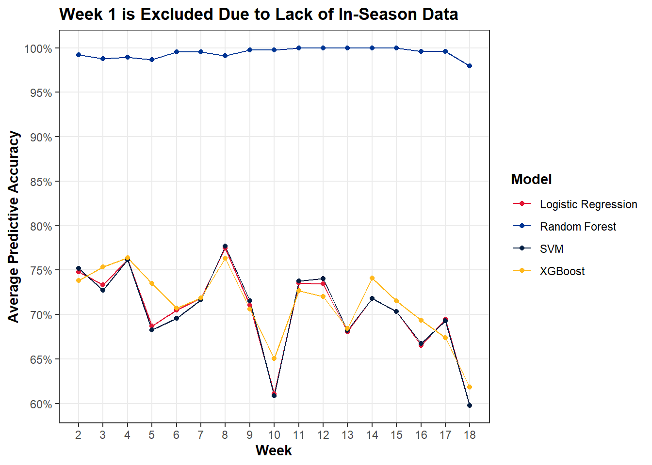
merged$log_preds <-predict(log_fit, merged, type ="prob")[,2]merged$rf_preds <-predict(rf_fit, merged, type ="prob")[,2]merged$rf_preds2 <-ifelse(merged$rf_preds >=0.5, 1, 0)merged$sv_preds <-predict(sv_fit, merged, type ="prob")[,2]merged$xgb_preds <-predict(xgb_fit, merged, type ="prob")[,2]merged %>%filter(week !=1) %>%mutate(log_class =ifelse(log_preds >=0.5, "Win", "Lose"),rf_class =ifelse(rf_preds >=0.5, "Win", "Lose"),sv_class =ifelse(sv_preds >=0.5, "Win", "Lose"),xgb_class =ifelse(xgb_preds >=0.5, "Win", "Lose")) %>%mutate(log_right =ifelse(win == log_class, 1, 0),rf_right =ifelse(win == rf_class, 1, 0),sv_right =ifelse(win == sv_class, 1, 0),xgb_right =ifelse(win == xgb_class, 1, 0)) %>%# By Week, Calculate Predictive Accuracygroup_by(week) %>%summarise(log_week_right =mean(log_right),rf_week_right =mean(rf_right),sv_week_right =mean(sv_right),xgb_week_right =mean(xgb_right)) %>%# Pivot to Color by Model Typepivot_longer(cols =starts_with("log_week_right"):starts_with("xgb_week_right"),names_to ="Model",values_to ="Accuracy") %>%mutate(Model =recode(Model,log_week_right ="Logistic Regression",rf_week_right ="Random Forest",sv_week_right ="SVM",xgb_week_right ="XGBoost")) %>%ggplot(aes(x = week, y = Accuracy, color = Model)) +geom_line() +geom_point() +scale_x_continuous(breaks =2:18) +scale_y_continuous(breaks =seq(0.6, 1, by =0.05),labels = scales::percent) +scale_color_manual(values =c("Logistic Regression"="#e31837", "Random Forest"="#003594", "SVM"="#041e42", "XGBoost"="#ffb81c") ) +labs(title ="Week 1 is Excluded Due to Lack of In-Season Data",x ="Week",y ="Average Predictive Accuracy",color ="Model") +blog_theme() +theme(plot.title =element_text(face ="bold"), legend.title =element_text(face ="bold") )
Average In-Sample Predictive Accuracy by Model Over NFL Weeks
Like a lot of things in the world of data science, when you plot the data expecting answers, you actually just get a lot more questions. While these report in-sample results (in contrast to cross-validated out-of-sample accuracy metrics… so take these accuracy numbers with a grain of salt), I still would have expected an upward trend over the NFL season, but nope! And there’s other interesting things as well… like how three of the models have a crazy dip in predictive performance in week 10. Don’t really know what that’s about. Well, even if the plot doesn’t support my diagnosis and prescription all that well, I’m convinced that pursuing a modeling strategy that incorporates prior information and domain knowledge would probably result in less “Saints over Cowboys” and “Vikings over 49ers” predictions.
Setting Up My Workflow
Lastly, I want to document how I’m going to go about creating predictions every week. After all, I’ve collected data and trained some models, but there is no magic button I can press that will just sequentially update everything every week throughout the remainder of the NFL season. The following code chunk walks through my “workflow” so to speak.
Now that I’ve created this, I hope that clicking “Run” now serves as the magical button that I just have to click and I get new predictions every week. We will see how this goes, as I’m sure there’s some bug/dependency I’m missing.