Testing Facebook’s {siMMMulator} Package for Marketing Data Simulation
causal inference
marketing
simulation
Simulating the data that you want by hand is always a task much easier said than done. As a result, I never turn away from a package designed to make simulation easier. As usual, there’s trade-offs between manually simulating and using customized softwares so I wrote up this blog to test out a neat looking simulation tool designed for marketing/MMM settings.
Published
December 16, 2025
Code
pacman::p_load("tidyverse", # Data Manipulation and Visualization"siMMMulator", # Simulating Marketing Data for MMMs"scales", # Scaling for Data Visualizationinstall =FALSE)# Define a Custom Themeblog_theme <-function() {theme_bw() +theme(panel.grid.major =element_line(color ="gray80", size =0.3),panel.grid.minor =element_blank(),panel.border =element_blank(),plot.background =element_rect(fill ="white", color =NA),plot.title =element_text(face ="bold", size =16, margin =margin(t =0, r =0, b =15, l =0)),axis.title.x =element_text(face ="bold", size =14, margin =margin(t =15, r =0, b =0, l =0)),axis.title.y =element_text(face ="bold", size =14, margin =margin(t =0, r =15, b =0, l =0)),strip.text =element_text(face ="bold"),axis.text.x =element_text(face ="bold", size =10), axis.text.y =element_text(face ="bold", size =10), axis.ticks.x =element_blank(), axis.ticks.y =element_blank(), strip.background =element_rect(fill ="grey80", color =NA),legend.title =element_text(face ="bold", size =14),legend.text =element_text(face ="bold", size =10, color ="grey25"), )}# Establish a Custom Color Schemecolors <-c("#0a697d","#0091af","#ddb067","#c43d56","#ab2a42","#A9A9A9")
Why Simulation Is So Important (and Hard…)
In any causal research endeavor, simulation is your friend. “What effect did this media mix have on sales?” That’s the motivating question behind marketing, but it’s incredibly challenging to answer. We attempt to answer this question by employing advanced statistical techniques and assuming (sometimes plausible) assumptions. But our assumptions are often wrong and our statistics are often poorly implemented. So how can you tell the difference between a good research design that can answer the business question and a research design that cannot? After all, either will produce numbers that can be dressed up in the mystique of fancy, esoteric math and engaging visualizations. If I’m a stakeholder, how am I to know which numbers are actionable and which results should not be treated as actionable?
This is where simulation shines. With a simulation analysis, you can manually create artificial marketing data with media/marketing effects hard-coded into the data (we would call this the data generating process). In doing so, we know what the effects are because we specified them. Then, we can test a number of different research designs on the simulated data to figure out which research design gets the closest to the truth. The leap that we make is that, if a given research design was able to estimate the true effect in the simulated data, then it should estimate the true effect in the real data.
Now, such an assumption isn’t a guarantee, because the ability to make inferences about your actual data generating process from your simulated data is dependent on how much your simulated data is like your real data. If the two are generated by totally different data generating processes, the quality of research designs could vary between the two data sets. There are no magic solutions when trying to do causal inference, but simulation will typically give you more information than what you had before the simulation analysis. As a result, if you take the time to think about the causal structures that generated your data, you’ll have a much more useful simulation analysis.
While thinking about your data generating process requires a good amount of effort, manually simulating data can also be a bit of a pain. As it turns out, when you’re in full control of how a data set is created, it’s super easy to get data that looks totally wrong. Much like programming, if you tell the computer to do something un-intuitive, it will do it and it won’t tell you that it’s a bad idea. If you define a data generating process that is going to produce un-intuitive results, your program will produce it and you’ll have to find out how ridiculous it is (and debug) on your own.
Because of this, I’m always interested in packages that attempt to make simulation easier. And that’s what this blog is all about. We’ll be taking a look at Facebook’s {siMMMulator}package designed to simulate data that you would use in a marketing/media mix model (MMM). The goal is to thoroughly explore its capabilities and (potentially) evaluate any limitations. In fairness to the developers of the package, they did a great job walking through how to use this package so I recommend checking that out as well!
Step 0: Define Basic Parameters
{siMMMulator} works by a series of building blocks. You follow a set order of commands (the commands are literally outlined for you… step_0, step_1, etc.) and, by the time you hit step 9, you have your simulated data set! Step 0 is pretty easy. You just establish the type of channels you’re interested in, the length of time covered in the data, each channel’s conversion rate and the amount of money made from each conversion.
Let’s walk through each argument in Step 0. The basic parameters in this blog will follow closely with those established in the package’s step-by-step user guide. Here, the only meaningful change I am making is adding more years of simulated data.
years: This just specifies the number of years that are simulated in the data set.
channels_impressions: This is just a collection of strings that can be named anything but are designed to store channels whose metrics of importance are impressions. You do not have to populate this argument if you are not interested in simulating channels that do not track impressions.
channels_clicks: This is the exact same thing as channel_impressions but just for channels whose metrics of importance are measured in clicks instead of impressions.
frequency_of_campaigns: This controls both how often campaigns occur and how long they last. In this case, I am telling my data generating process that campaigns roll out every 2 weeks and last 2 weeks.
true_cvr: This tells us the conversion rate for each channel. Conversion rates are stored in the same order that they appear in channel_impressions and channel_clicks. In this case, the conversion rate for Facebook is 1/1000 impressions, the conversion rate for TV is 2/1000 impressions, and the conversion rate for Paid Search is 3/1000 clicks.
revenue_per_conv: This establishes how much money is made per conversion.
start_date: This just sets the start date for the data.
Limitations
It doesn’t look like {siMMMulator} allows for varying campaign frequencies and revenue per channel. You can only enter one type of campaign frequency in the frequency_of_campaign argument and 1 revenue amount in revenue_per_conv. Personally, this seems like a really big limitation. If universal campaign frequencies and ad revenues make sense for your business context, then sure, this isn’t a problem, but I’m not sure how realistic that is. If there is known wide variation between media campaign frequency/revenue, you might want to look elsewhere for a simulation analysis.
base_p: This is your baseline sales at the start of the period or, in other terms, what your sales would be without any spend on any of the media specified in Step 0.
trend_p: The overall trend on how baseline sales will grow over the entire period of the data set. This is something that is good to play around with and graphically inspect (which we will do below!)
temp_var: This is used to “inject seasonality” into the data. Much like trend_p, this is something that is good to iterate and experiment with.
temp_coef_mean: This determines how important seasonality is for sales.
temp_coef_sd: This value will determine how much variability exists with the importance of seasonality on sales.
error_std: This is the amount of noise that is added to baseline sales. The greater this number is, the more noisy your baseline sales will be.
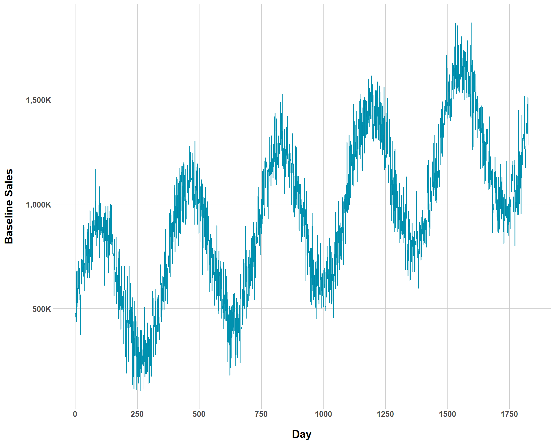
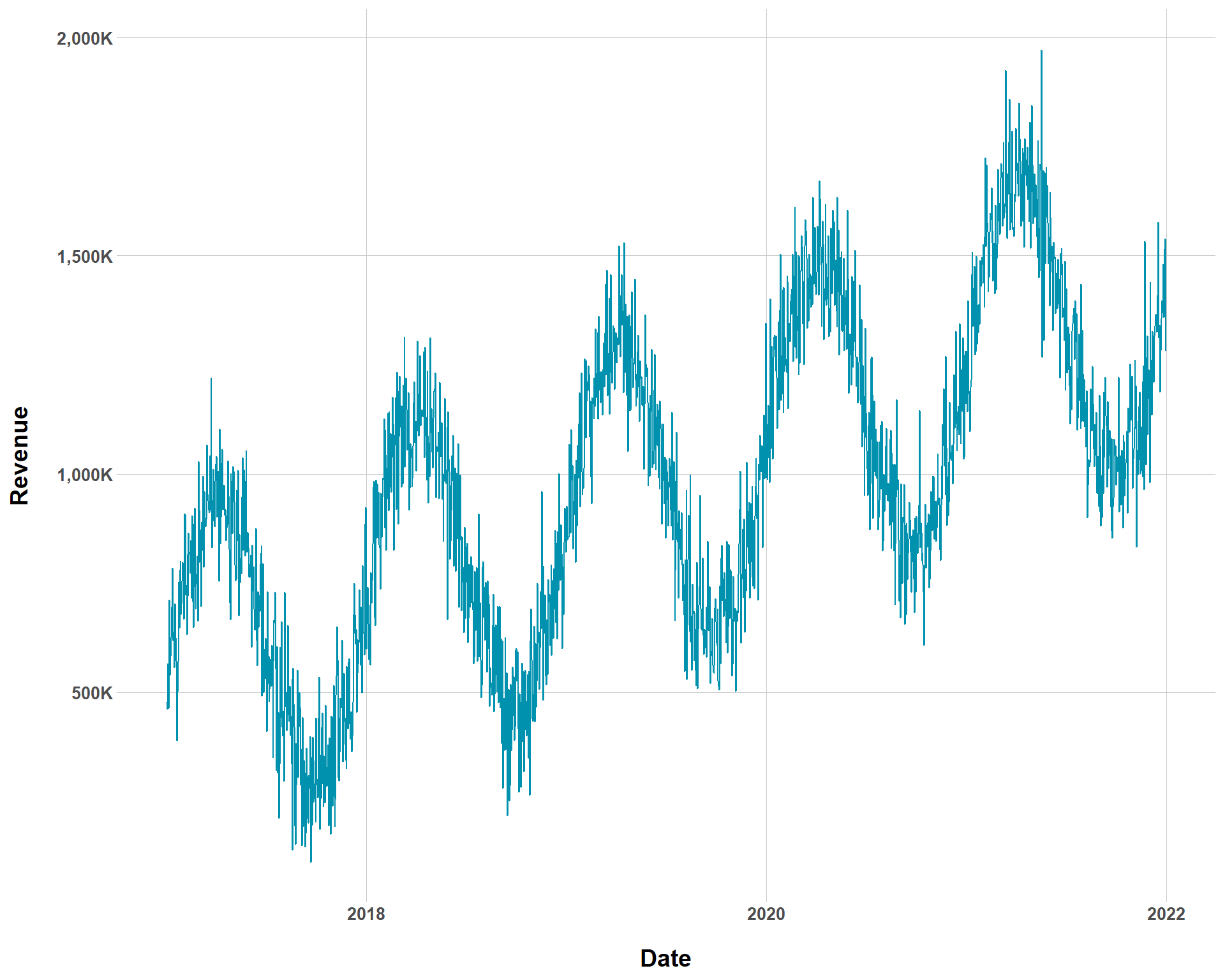
{siMMMulator} has some built in features that allow you to inspect what your data looks like as you go down the simulation pipeline. Given what we have so far, we get the follow time series.
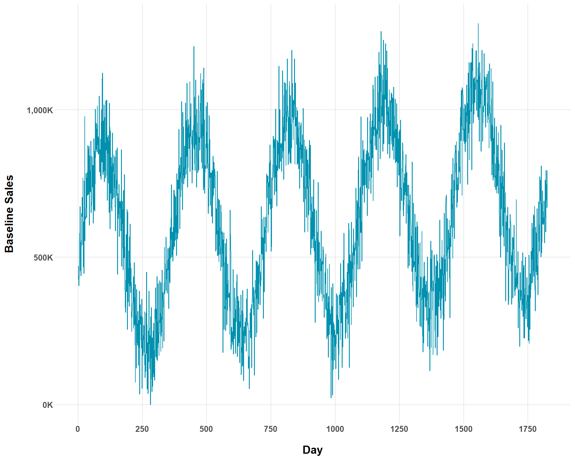
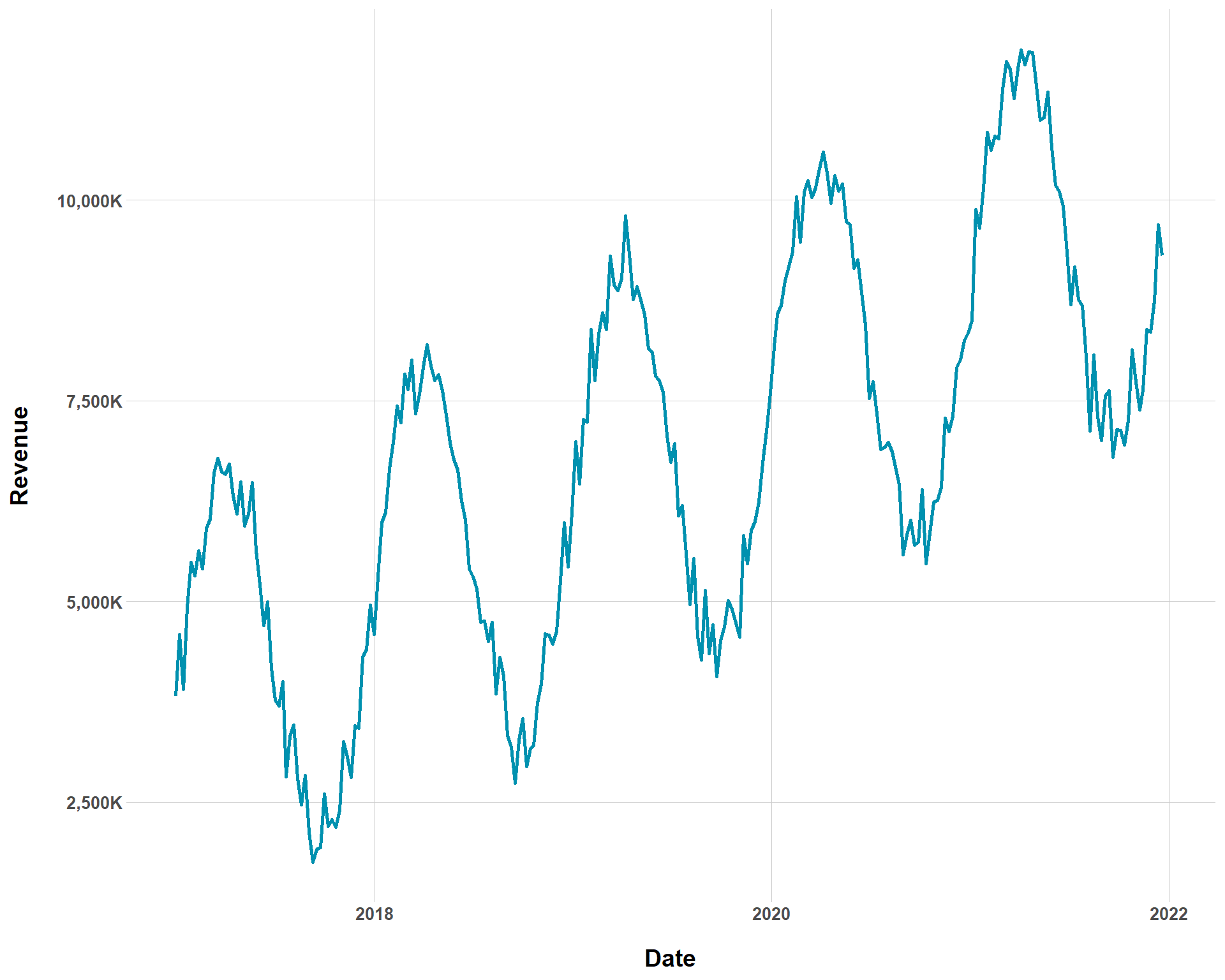
Now, we can vary trend_p and see how much baseline sales change over time. I’m going to decrease trend_p substantially to really make the change apparent.
You can see now that the overall rate of baseline growth is now much smaller than before. But we could complicate our ability to even visually determine baseline growth by increasing the amount of noise to the our baseline sales.
Baseline Sales with Smaller Baseline Growth and Greater Noise
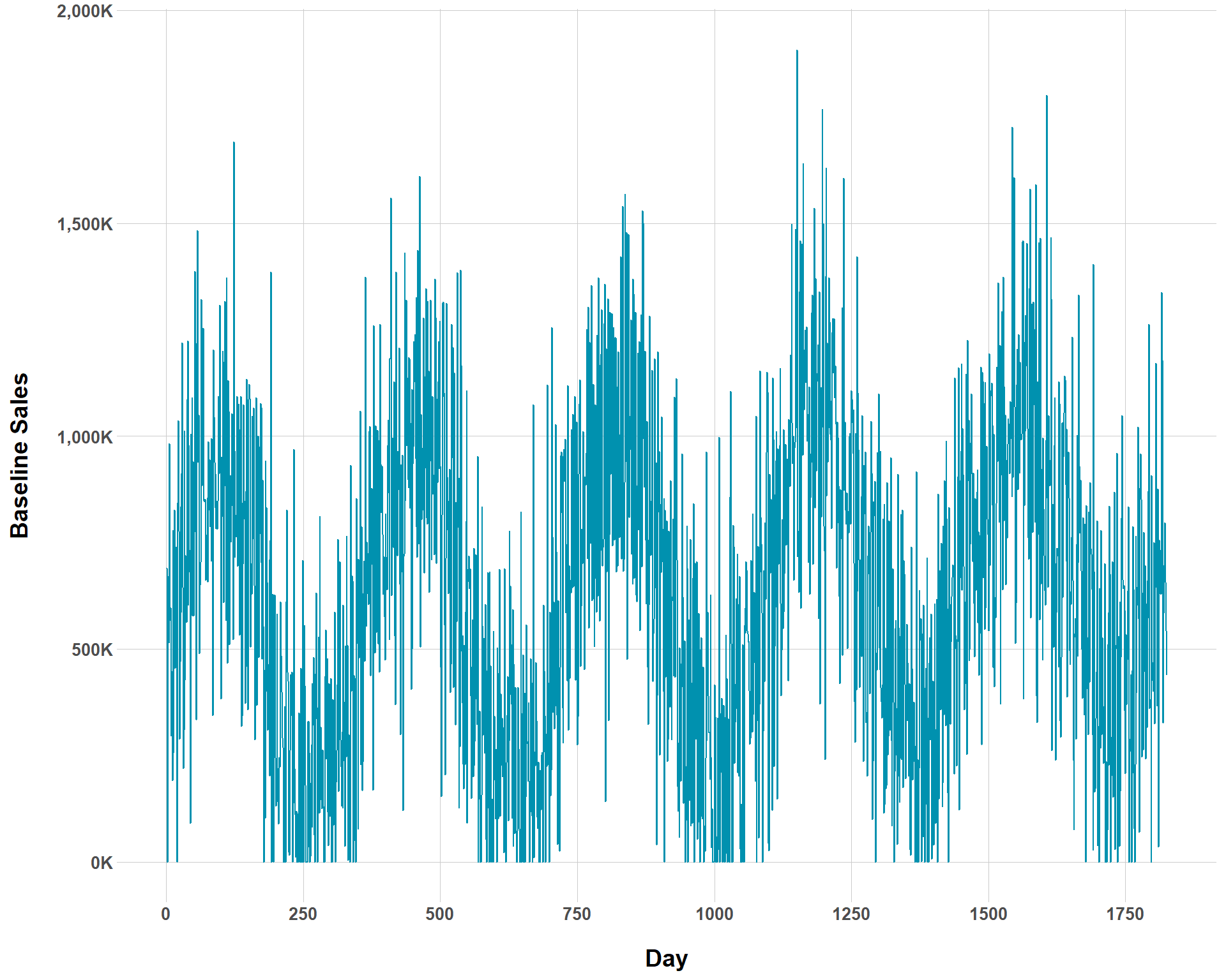
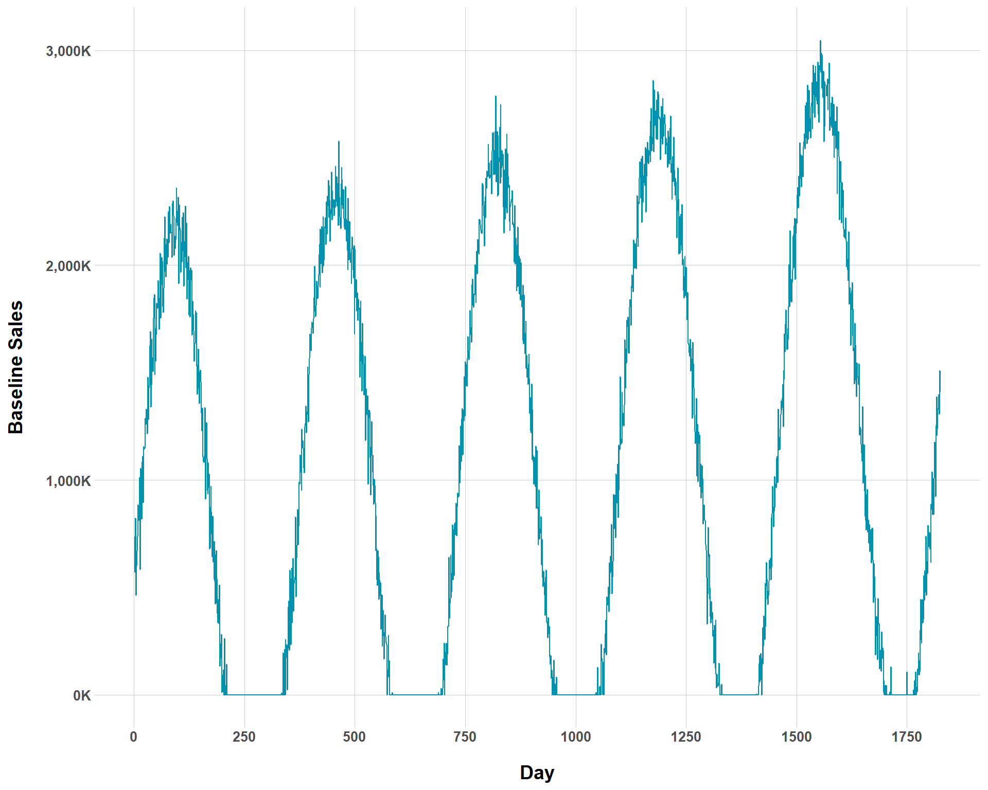
Hey, not everything can be a tidy toy data set. We can also mess with how sharp seasonality swings are in our data. By setting the temp_var to higher values, we can see steeper changes in sales at different times throughout the years.
Related, but still different, we can control the effect of seasonality on sales. While temp_var basically models the height of the swing, temp_coef_mean and temp_coef_sd directly establish the average effect of seasonality on sales. Showing what changing these values does to baseline sales will probably be helpful in distinguishing them from temp_var.
Baseline Sales with Sharp Seasonality Swings and Large Seasonality Effects
Obviously, this is extremely hyperbolic data, but that’s the fun (and utility!) of playing around with simulated data. For most businesses, such seasonality assumptions are not realistic (this might be accurate for ski resorts?). I’m intentionally being extreme in the values set to get an idea of what each thing does in the argument.
But, even with all of this, we’re still just at Step 1. We’ve only simulated baseline sales. We haven’t yet got to simulating media spend and effects.
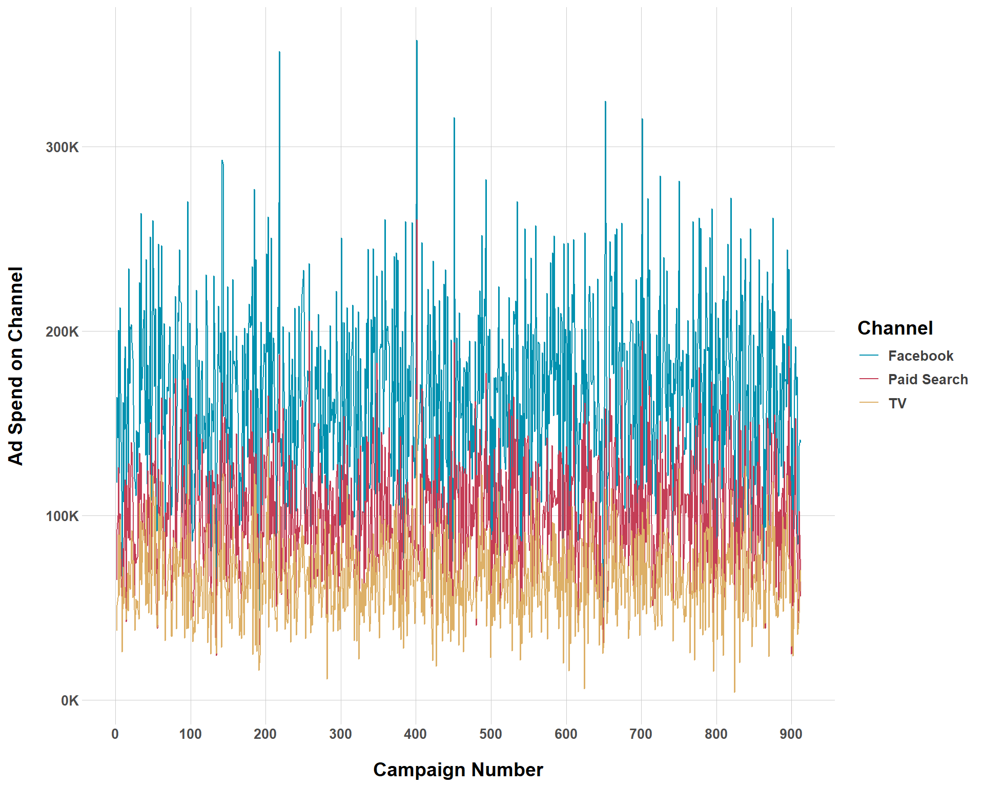
Above is a plot showing ad spend by channel over each campaign. Remember that we set our campaign to occur every 2 weeks so the x-axis will not reflect the total number of days in a 5-year period. Let’s walk through each argument to see how this ad spend was generated.
my_variables: This is your object of baseline variables that were produced in Step 0.
campaign_spend_mean: This reflects the average amount of money that is spent on all media campaigns throughout the entire period that the data set covers. Here, you do not need to worry about how that budget is allocated between different channels. That is what the max_min_proportion_on_each_channel argument is about.
campaign_spend_std: This is how you can make your campaign_spend_mean have greater/less variation.
max_min_proportion_on_each_channel: Modifying this is how you allocate the media budget between different channels. Each channel has a minimum and a maximum percent of the budget that they can receive. For example, the least that Facebook receives in the budget is 45% and the most is 55%. The least that TV receives is 15% and the most is 25%. But, what about paid search? Well, you don’t have to specify that because we are working with percentages. If Facebook takes up 45-55% and TV takes up 15-25% then paid search must take up 20-40% of the budget (45% + 15% + 40% = 100% or 55% + 25% + 20% = 100%.) Basically, the amount of numbers populated in this argument will always be (\(k\) (number of channels) - 1) * 2.
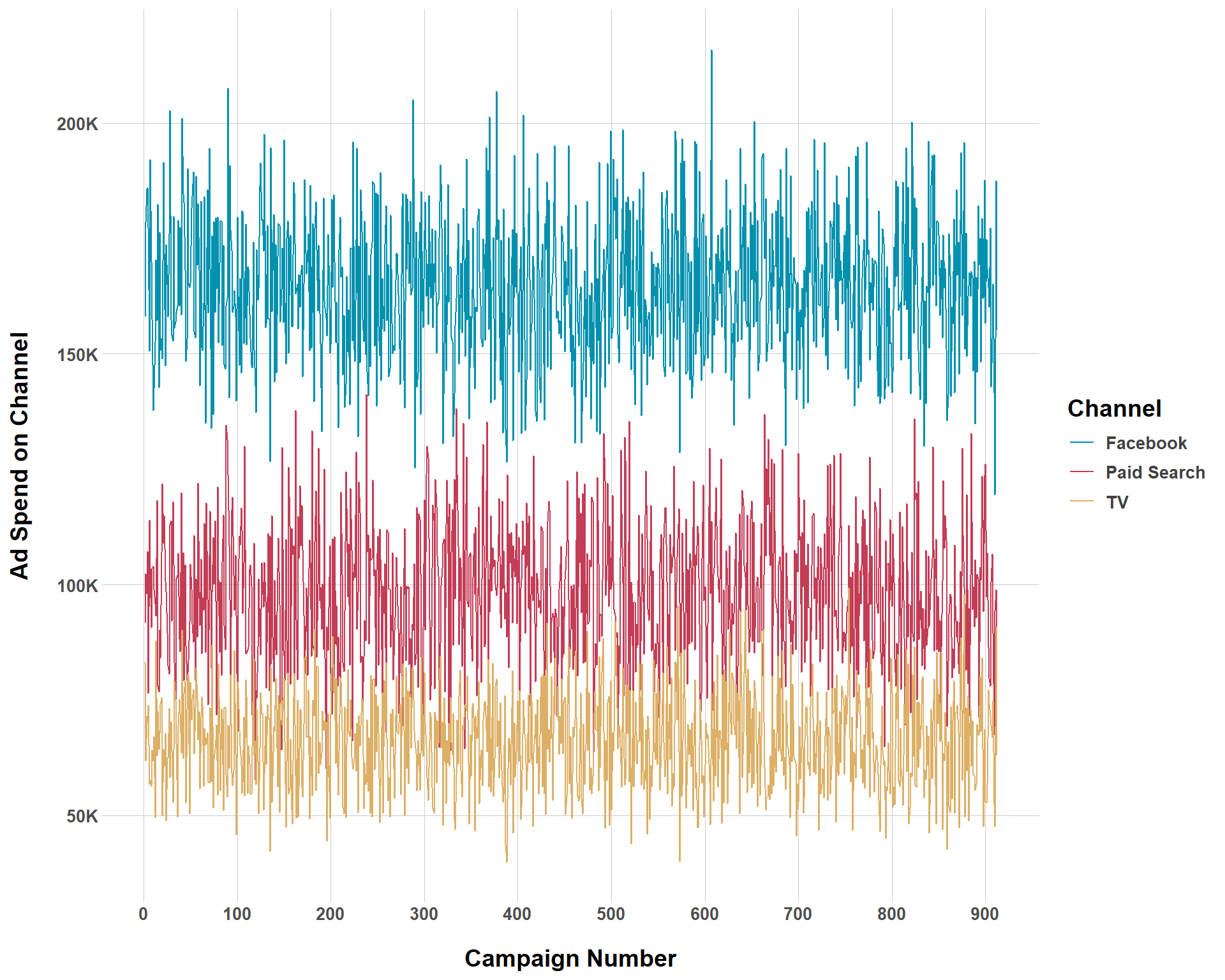
And just for fun, let’s see what ad spend looks like if we make our budget less noisy.
And that checks out! With less variation, there is clearer distinction between channels concerning which get greater budget allocation.
Step 3: Generate Media Variables
Now that we have our baseline information and simulated ad spend, we’re in good shape to move on to Step 3 and begin to simulate channel activity. In this step, we specify what the cost per impression/click is for each channel.
Computation Time
I’m not really sure why but Step 3 took considerably longer to run than any of the other steps so far. Still, it didn’t take a super long time, just around a minute. But it was long enough that I thought I should include a brief note because all the other steps so far took about 1-2 seconds.
true_cpm: This sets the true cost per impression (CPM) for each channel where impressions are a relevant metric. These numbers are ordered in accordance with how channels were specified in Step 0. For channels where this metric is not relevant, NA is used.
true_cpc: This sets the true cost per click (CPC) for each channel where clicks are a relevant metric. These numbers are ordered in accordance with how channels were specified in Step 0. For channels where this metric is not relevant, NA is used.
mean_noisy_cpm_cpc: This sets the mean of the normal distribution that is used to add noise to CPM/CPC.
std_noisy_cpm_cpc: This is the second part of the noise generation process that sets the standard deviation of the normal distribution that noise for CPM/CPC is produced from.
Step 4: Generate Noisy CVRs
Step 4 takes us back a bit to something we did in Step 0. There, we already established conversion rates for each channel. But conversion rates are not static, so Step 4 allows us to inject some statistical noise to our conversion rates.
mean_noisy_cvr: Mean of the normal distribution used to add noise to our CVRs.
std_noisy_cvr: Standard deviation of the normal distribution used to add noise to our CVRs.
Step 5: Transforming Media Variables
Step 5 is a bit more complex because, up to this point, we have built in assumptions into our data set that the effect of media on revenue is linear. But this is for sure not true. For any simulation analysis to be helpful, it needs to capture the (potentially complex) realities that occur in the actual data generating process. For Step 5, we apply adstock and diminishing returns to our media effects. But first, we execute Step 5a which pivots the data to a daily format.
Now that this done, we can simulate adstock. For those unfamiliar, this is basically the lagged effect of a given campaign. That is, even if a campaign ends, it still likely has some “decayed” effect over time. A TV commercial campaign can end, but I can still think about it after it stops fielding and that can influence my purchasing decisions. Again {siMMMulator} makes this very easy, where we specify a number between 0 and 1 that controls how long the lagged effect lasts.
The 0.1, 0.2, and 0.3 refer to distinct lagged effects for each channel. Like all other steps in this process, the effects correspond to the channels in the order they were specified in Step 0.
Lastly, we can build in diminishing media effects to account for the fact that, as time goes on, increased/the same amount of spending for a given channel will not yield increased, or even the same level of results due to saturation. You can control diminishing returns via two parameters, alpha and gamma saturation (from Facebook’s Robyn). Alpha controls how steep the curve is (higher alpha models a more “S”-shaped curve which means the channel saturates more quickly while lower alpha values resemble a “C”-shape which denotes a more gradual rate until saturation). In other words, manipulating alpha changes how long it takes until a channel effect is saturated. Gamma controls the inflection point or, the level of spend when a channel hits saturation. The larger that gamma is, the later the inflection point occurs.
To put this all into a simpler example, say that we set alpha to be lower and a gamma value to be high. Doing so would model our saturation point to occur late and the rate that we approach that saturation point to be very gradual. In contrast, if we reversed it and alpha was high and gamma was low, we would be modeling a scenario where the saturation point occurs very early on and we approach it rapidly.
Weird Warning
When you run step_5c_diminishing_returns(), you get a crazy long warning message that repeats “lengthWarning: longer object length is not a multiple of shorter object” over and over and over again. You won’t see it in this blog because I’m suppressing it, but I get it every time. I’m not sure why this is the case, and it doesn’t seem to produce any problems, but that’s something to be aware of.
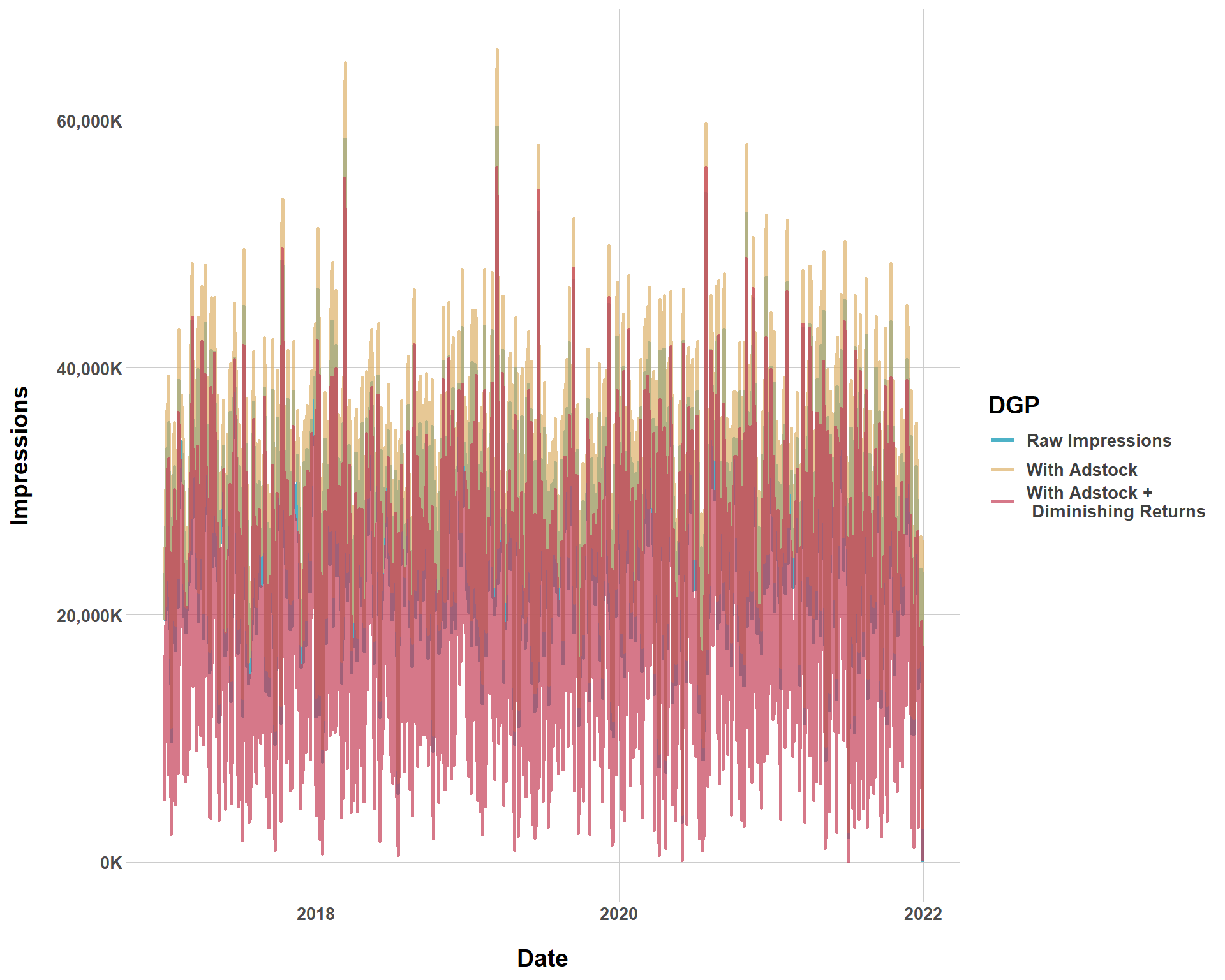
So we’ve worked with adstock and diminishing returns, messing around with alpha, gamma, and lambda. But this still has all been a bit abstract. {siMMMulator} does not provide built in plotting functions to plot these effects like they did in Steps 1 and 2. But, we still get a data frame that we can play around with from our dim_returns data frame. Let’s start by looking at how impressions for the Facebook channel in particular changes when manipulating alpha, gamma, and lambda. We’ll start by looking at how impressions for Facebook change without adstock or diminishing returns, only with adstock, and with adstock and diminishing returns.
Facebook Conversions with Different Data Generating Processes
It’s kind of hard to tell, but we see that the data generating process with diminishing returns (unsurprisingly) has the most downward impressions while the DGP with adstock but without diminishing returns has the most upward impressions. This all totally makes sense. A DGP with just adstock means that every campaign has decaying effects, with means every campaign at \(t-1\) gets a little more extra boost from the campaign at time \(t\). However, once we introduce diminishing returns, we get… diminishing returns, which means we are modeling less impressions.
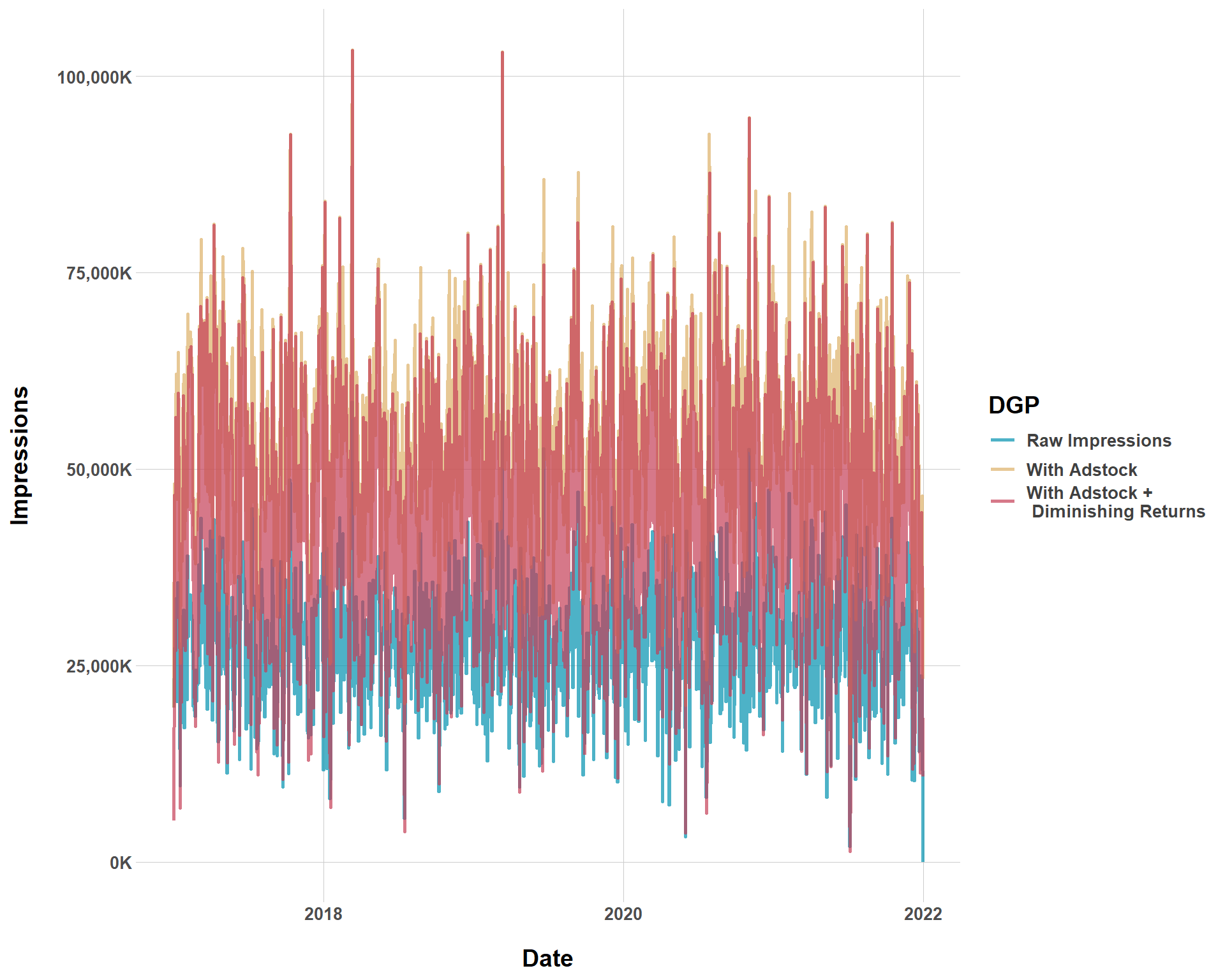
Now, let’s get crazy and simulate another DGP with very long lagged effects and very steep and immediate diminishing returns. Again, this is just for fun and familiarity with the package.
In Step 7, we “do final calculations for all the variables that we need for the final data frame”. There’s nothing customizable that you do here, it’s just a procedural step.
Again, this a very easy, self-explanatory step. In the guide, the author does not store the results in a data frame and it doesn’t seem like the results from Step 8 are built into the final step. However, this is still an important step because these results are our baseline truth for our most important metric (ROI). Again, we want that baseline truth so we can compare it to the results we’d get from an MMM we might use to see how biased it is. I won’t be testing any model’s in this blog, so I’m just going to run this and not use it in this blog, but this step is still very important.
Overall, this package certainly makes simulation easier! But it does have some of the natural and universal limitations that any package does. But, that is the price you pay for convenience.