Understanding the Piranha Problem and Navigating Statistical Reporting In Light of Your Cannibalistic Effects

It is often said that ‘there are no free lunches in causal inference’. I am not here to dispute that claim. In fact, this inconvinient fact is present in ways that we don’t often think of. Check out this post to learn about the so-called ‘Piranha Problem’ and why it is probably very important to understand for your research and what to do about it.

pacman::p_load(
  "tidyverse", # Data Manipulation and Visualization
  "marginaleffects", # Marginal Effects
  "tinytable", # Reporting Tabular Results
  "scales", # Plotting Percentages
  install = FALSE
)

# Define a Custom Theme
blog_theme <- function() {
  theme_bw() +  
    theme(
      panel.grid.major = element_line(color = "gray80", size = 0.3),
      panel.grid.minor = element_blank(),
      panel.border = element_blank(),
      plot.background = element_rect(fill = "white", color = NA),
      plot.title = element_text(face = "bold", size = 16, margin = margin(t = 0, r = 0, b = 15, l = 0)),
      axis.title.x = element_text(face = "bold", size = 14, margin = margin(t = 15, r = 0, b = 0, l = 0)),
      axis.title.y = element_text(face = "bold", size = 14, margin = margin(t = 0, r = 15, b = 0, l = 0)),
      strip.text = element_text(face = "bold"),
      axis.text.x = element_text(face = "bold", size = 10), 
      axis.text.y = element_text(face = "bold", size = 10), 
      axis.ticks.x = element_blank(), 
      axis.ticks.y = element_blank(), 
      strip.background = element_rect(fill = "grey80", color = NA),
      legend.title = element_text(face = "bold", size = 14),
      legend.text = element_text(face = "bold", size = 10, color = "grey25"),
    )
}

# Establish a Custom Color Scheme
colors <- c(
  "#0a697d",
  "#0091af",
  "#ddb067",
  "#d4924a",
  "#c43d56",
  "#ab2a42",
  "#A9A9A9"
)

set.seed(1234)

# Turn Off Scientific Notation
options(scipen = 999)

Our Model of Scientific Progress is Messed Up…

Whether we are aware of it or not, most of us (and especially our less technically-inclined audiences/consumers of our research) have a plain, additive model of scientific research. In other words, there is some outcome or metric of interest and, whether your are in consulting work or doing academic research, the idea is to find “levers” that the client/policymakers can pull to induce some desired change in the outcome of interest. The problem is that we often assume that there’s tons of levers out there and that pulling one lever results in a substantive, unique effect.

In other words, we think of science like this:

\(Y = \text{BigEffect}*X1 + \text{BigEffect}*X2 + \text{BigEffect}*X3 + ...\)

This is not the most natural or realistic way to think about an incredibly interactive world. However, we are all pressured into it by external forces. In consultancy, clients are constantly looking for new “levers” to pull, assuming (most of the time, erroneously) that existing, long-established levers are well understood and that the only way to keep improving their KPIs are to invest in the testing of new, less-studied levers. In academia, there is a not-so-hidden structural push for each researcher who wants to make a name for themselves and to build a career by finding their “pet” independent variable and to test it against every outcome under the sun. Most of the time, the big dog variables (economic development, socio-economic status, etc.) have already been taken decades ago, so researchers mine for increasingly niche levers.

These forces lead to bad science and misleading statistical output, even though most of us researchers have no insidious intentions. In the real world, dozens of effects, let alone hundreds that are marketed in social scientific research, cannot all have large and stable effects. If any variable (besides the obvious heavy-hitters) has an effect on \(Y\), it is probably really small and is contextually highly variable to interactions with other causes of \(Y\). Tosh et al. (2024) flagged this realization and dubbed the issue the “Piranha Problem”, with the name originating from “the folk belief that if one has a large number of piranhas (representing large effects) in a single fish tank, then one will soon be left with far fewer piranhas.”

In this blog post, I aim to walk through some simulated examples to help illustrate 1) that this is a real problem, 2) why this problem exists, and 3) what to do in light of this problem. My main takeaways are two-fold. First, we should probably abandon the naive assumption that is implicit in most of our statistical reporting of a single average effect size. Even under the strongest of assumptions that these effects are unbiased and close to the truth (a massive uphill battle in its own right), that does not mean that the average effect is informative across realistic contexts in the real world. Second, novel scientific research should be less interested in finding “new levers” and more interested in testing how existing, “well-understood” levers interact with each other.

Simulating DGPs

To walk through the Piranha Problem, I am going to simulate 4 different data generating processes. I am going to make a HUGE assumption in each scenario that there is no unobserved/unadjusted confounding. This is basically never true, but I am doing this to specifically focus on how we can mislead with our reporting, even when we have acheived the Herculean task of dealing with confounding. In other words, I’m giving the status-quo approach to science a handicap because residual confounding compounds problems.

For the sake of sticking to my “levers” illustration, I’m going to simulate an imagined DGP that is very manipulable. I simulate 4 different cross-sectional data sets, each with an \(n\) of 10,000 people. The outcome of interest in a binary indicator of whether an individual has subscribed to a service or not. There are five exposures of interest: whether an individual received a free trial, whether an individual received a promotional deal, whether an individual was personally recommended the service, whether the individual was contacted by a member of the sales team, and whether an individual was exposed to a targeted advertisement. All exposures are simulated “as-if” they are random, because I’ve built in the assumption that we’ve removed confounding bias from the treatment assignment.

Each scenario includes different (increasingly realistic) rules about the DGP. Scenario 1 simulates a world in which there are multiple large and stable effects. This world is very improbable. Scenario 2 simulates a world in which there are multiple large effects and they interact with each other to boost the effect size. While the interactivity component is realistic, the idea that they are all large is unrealistic. Scenario 3 simulates a world where there are multiple large effects, but they interact with each other and depress each other’s effect sizes, which is getting us closer to the real world. Scenario 4 is the most realistic simulation of how causal effects operate in the real-world; there are a couple of larger effects, several smaller effects, and they interact with each other in different ways. Scenario 4 will really help shed some light on why the additive model of novel research and only interpreting non-interacted average effects is problematic.

Scenario 1: Multiple Large and Stable Effects

Scenario 1 is implicitly what most people believe in. They, of course, do not denounce the existence of small and/or interactive effects, but they do believe there is a buffet of large effects that persist in size and magnitude across all sorts of environmental contexts. This is a comfortable view for a researcher who wants to show that their pet theory is correct or a stakeholder who believes that there are multiple, undiscovered levers that will finally get those KPIs to where they need to be, but it is an unrealistic one. In the simulation code below, I am simulating, for each individual, the probability that they have subscribed for the service of interest with a baseline 25% probability of subscribing. The five variables of interest have large and stable effects, ranging from a 20 percentage point to a 30 percentage point increase in the Pr(Subscribed)

set.seed(1234)

n <- 10000

scen1_data <- data.frame(
  free_trial = rbinom(n, 1, 0.2),
  promotion = rbinom(n, 1, 0.4),
  personal_rec = rbinom(n, 1, 0.1),
  sales_contact = rbinom(n, 1, 0.15),
  targeted_ad = rbinom(n, 1, 0.3)
)

# Simulate Subscribed on the Probability Scale
scen1_data$p_subscribed <- with(scen1_data,
  0.25 + 0.3*free_trial + 0.25*promotion + 0.2*personal_rec + 0.2*sales_contact + 0.23*targeted_ad)

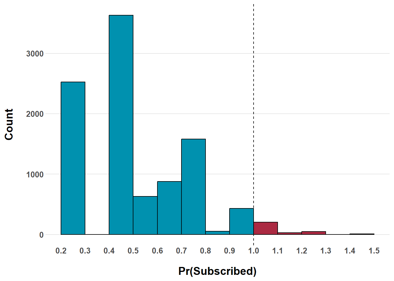
Below, we can already see an issue with these assumptions. In this case, assuming multiple large and stable effect sizes leads to impossible outcome values.¹ Shaded in red are individuals whose Pr(Subscribing) is greater than 1 (100%). These are theoretically impossible values to obtain, but this is part of the reality of assuming multiple large and stable effects. If, in some way, these large effects do not interact and depress the effects of other variables, they simply add up to impossible values.

ggplot(scen1_data, aes(x = p_subscribed, fill = after_stat(x <= 1))) +
  geom_histogram(binwidth = 0.1, boundary = 0, color = "black") +
  scale_x_continuous(breaks = seq(0, 1.5, by = 0.1)) +
  labs(
    x = "Pr(Subscribed)",
    y = "Count"
  ) +
  scale_fill_manual(
    values = c("TRUE" = colors[2], "FALSE" = colors[6]),
    guide = "none"
  ) +
  geom_vline(xintercept = 1, linetype = "dashed") +
  blog_theme() +
  theme(
    panel.grid.major.x = element_blank(),
    panel.grid.minor.x = element_blank()
  )

Distribution of Probabilities with Multiple Large and Stable Effect Sizes

One could also find a similar issue with outcome variables on a different scale. For example, we could be interested in mortality (measured as age) for an outcome. Multiple large and stable effects might mean that, for some individuals, our model could predict that they would live to 150! Or, our outcome could the classic number of fish caught and we might find that, for some “lucky” folks, we predict they would catch 100 fish…

Regardless, the point still stands. Multiple large and stable effects either create impossible outcome values or, sampling from a distribution with a defined range, results in values being dropped from the analysis because the specified DGP created values that are impossible. The verdict then? Multiple large and stable effects are very unlikely in the real world…

Scenario 2: Multiple Large Effects That Interact and Augment Each Other

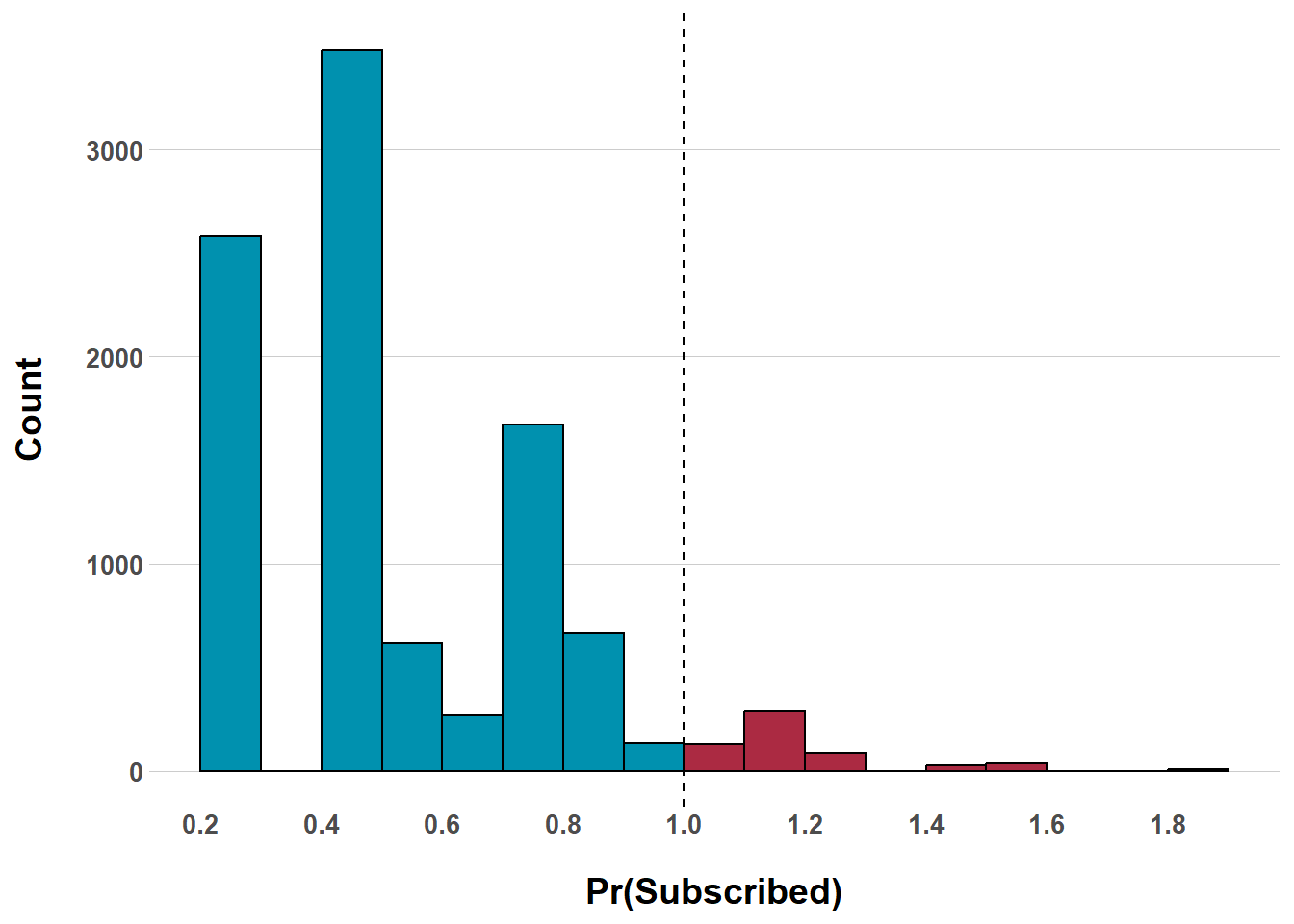
But what if we, instead, dropped the stability assumption and let the effects interact with each other? In Scenario 2, I’m going to simulate a DGP whose outcome should be obvious after the results in Scenario 1, but I’m still doing this to showcase that, if interactivity between effects exists, it needs to be negative, to some extent, to produce outcome values that are actually possible. Scenario 2 is going to produce some whacky results, because I have included multiple interactions between the lever variables that only increase the effectiveness on getting people to subscribe.

scen2_data <- data.frame(
  free_trial = rbinom(n, 1, 0.2),
  promotion = rbinom(n, 1, 0.4),
  personal_rec = rbinom(n, 1, 0.1),
  sales_contact = rbinom(n, 1, 0.15),
  targeted_ad = rbinom(n, 1, 0.3)
)

# Simulate Subscribed on the Probability Scale
scen2_data$p_subscribed <- with(scen2_data,
  0.25 + 0.3*free_trial + 0.25*promotion + 0.2*personal_rec + 0.2*sales_contact + 0.23*targeted_ad +
    free_trial*promotion*0.1 + free_trial*sales_contact*0.12 + personal_rec*free_trial*0.08 +
    personal_rec*targeted_ad*0.05 + promotion*sales_contact*0.07 + targeted_ad*sales_contact*0.03)

As expected, now we are seeing even more extreme and impossible results! Again, this is obvious, but I just wanted to drive home the point that assuming interactivity is not enough… If we are to assume multiple large effects, they, at the very least, need to interact with each other and depress the other effects.

ggplot(scen2_data, aes(x = p_subscribed, fill = after_stat(x <= 1))) +
  geom_histogram(binwidth = 0.1, boundary = 0, color = "black") +
  scale_x_continuous(breaks = seq(0, 2, by = 0.2)) +
  labs(
    x = "Pr(Subscribed)",
    y = "Count"
  ) +
  scale_fill_manual(
    values = c("TRUE" = colors[2], "FALSE" = colors[6]),
    guide = "none"
  ) +
  geom_vline(xintercept = 1, linetype = "dashed") +
  blog_theme() +
  theme(
    panel.grid.major.x = element_blank(),
    panel.grid.minor.x = element_blank()
  )

Distribution of Probabilities with Multiple Large and Augmented Interactions

Scenario 3: Multiple Large Effects That Interact and Depress Each Other

In Scenario 3, we are still sticking with the (unrealistic) assumption that all effects of interest are substantively large, but we are injecting some more realism into this simulation by letting the interactions all be negative. This should result in simulated outcomes that are more congruent with reality. Although, please note that these negative interactions are practical for the sake of demonstration and are not theoretically motivated (I have no clue if the effect of a personal recommendation is moderated negatively by receiving a free trial for a product/service).

scen3_data <- data.frame(
  free_trial = rbinom(n, 1, 0.2),
  promotion = rbinom(n, 1, 0.4),
  personal_rec = rbinom(n, 1, 0.1),
  sales_contact = rbinom(n, 1, 0.15),
  targeted_ad = rbinom(n, 1, 0.3)
)

# Simulate Subscribed on the Probability Scale
scen3_data$p_subscribed <- with(scen3_data,
  0.25 + 0.3*free_trial + 0.25*promotion + 0.2*personal_rec + 0.2*sales_contact + 0.23*targeted_ad +
    free_trial*promotion*-0.07 + free_trial*sales_contact*-0.06 + personal_rec*free_trial*-0.1 +
    personal_rec*targeted_ad*-0.08 + promotion*sales_contact*-0.05 + targeted_ad*sales_contact*-0.04)

# Convert Probability to Log-Odds
scen3_data$logit_p <- qlogis(scen3_data$p_subscribed)

# Simulate Binary Subscribed Outcome
scen3_data$subscribed <- rbinom(
  n, size = 1, prob = plogis(scen3_data$logit_p)
)

# Artificially Re-Code NAs to 1
scen3_data <- scen3_data |> 
  mutate(
    subscribed = ifelse(is.na(subscribed), 1, subscribed)
  )

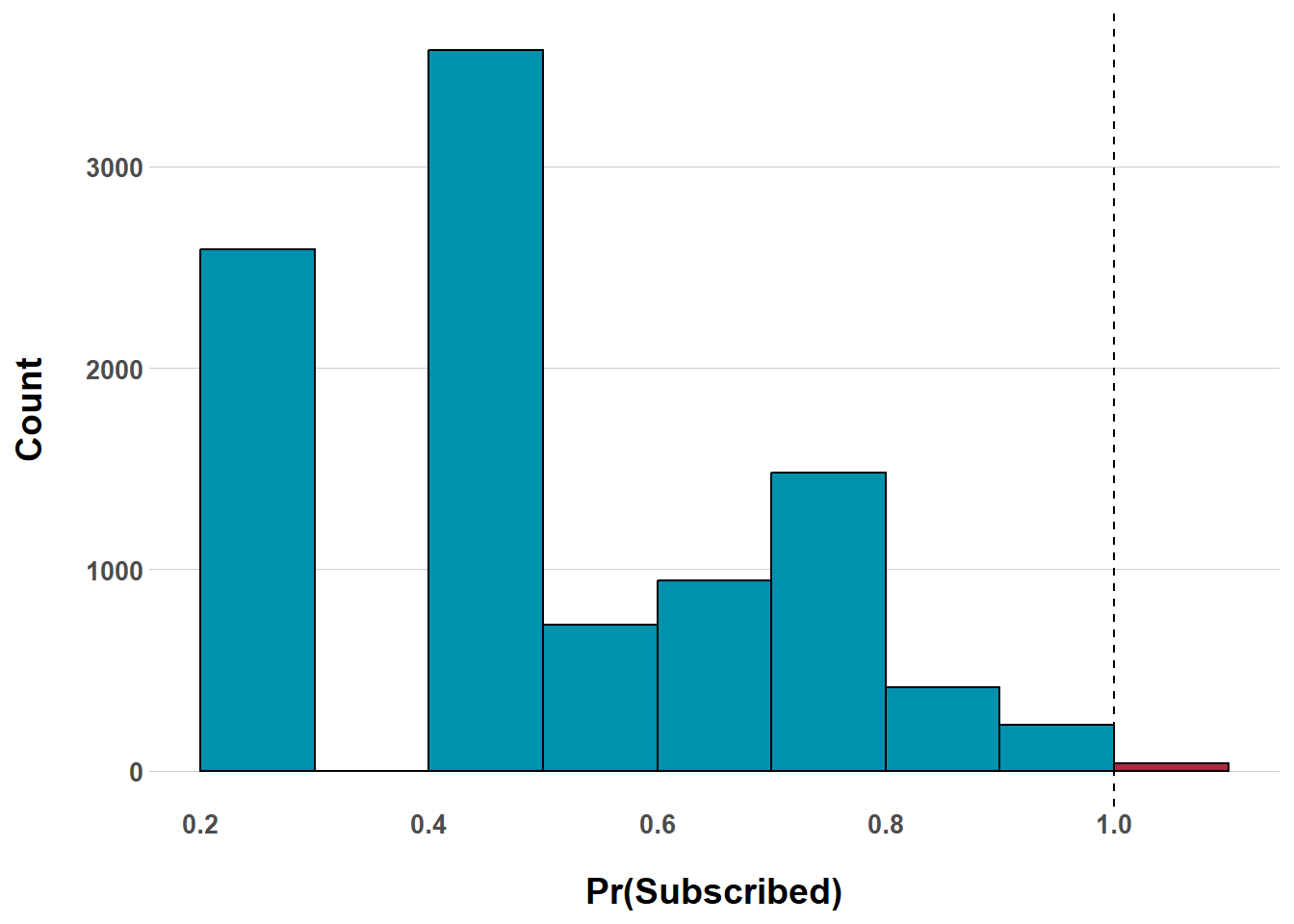
Okay, pretty good! There’s still a small amount of individuals with impossible probabilities, but this is much better than the prior two scenarios. One could imagine that, if many of these effect sizes were smaller, we would observe a world that is actually possible…

ggplot(scen3_data, aes(x = p_subscribed, fill = after_stat(x <= 1))) +
  geom_histogram(binwidth = 0.1, boundary = 0, color = "black") +
  scale_x_continuous(breaks = seq(0, 2, by = 0.2)) +
  labs(
    x = "Pr(Subscribed)",
    y = "Count"
  ) +
  scale_fill_manual(
    values = c("TRUE" = colors[2], "FALSE" = colors[6]),
    guide = "none"
  ) +
  geom_vline(xintercept = 1, linetype = "dashed") +
  blog_theme() +
  theme(
    panel.grid.major.x = element_blank(),
    panel.grid.minor.x = element_blank()
  )

Distribution of Probabilities with Multiple Large and Depressed Interactions

Also note that, just because the distribution of probabilities is almost within a possible range, that does not mean that we are out of the clear. While one part of the Piranha Problem is that, if multiple large and stable effects were true, they would produce an unrealistic/impossible outcome, the other part is that even unbiased average effects are still contextual.

We can demonstrate that below. For practical reasons, please note that I am re-coding probabilities > 1 to “1”. This is not correct… but we are technically working with impossible data anyways, so please just view this as a demonstration.

# Convert Probability to Log-Odds
scen3_data$logit_p <- qlogis(scen3_data$p_subscribed)

# Simulate Binary Subscribed Outcome
scen3_data$subscribed <- rbinom(
  n, size = 1, prob = plogis(scen3_data$logit_p)
)

# Artificially Re-Code NAs to 1
scen3_data <- scen3_data |> 
  mutate(
    subscribed = ifelse(is.na(subscribed), 1, subscribed)
  )

scen3_mod <- glm(subscribed ~ free_trial + promotion + personal_rec + sales_contact + targeted_ad, data = scen3_data, family = binomial(link = "logit"))

avg_comparisons(scen3_mod, variables = c("free_trial", "promotion", "personal_rec", "sales_contact","targeted_ad")) |> 
  mutate(truth = c(0.3, 0.2, 0.25, 0.2, 0.23),
         estimate = round(estimate, 2),
         term = recode(
           term,
           free_trial = "Free Trial",
           promotion = "Promotion",
           personal_rec = "Personal Rec",
           sales_contact = "Sales Contact",
           targeted_ad = "Targeted Ad"
         )) |> 
  select(
    `Lever Variable` = term,
    `Estimated AME` = estimate,
    `True Effect` = truth
  ) |> 
  tt() |> 
  style_tt(
    j = 2:3,
    align = "c"
  )

Lever Variable	Estimated AME	True Effect
Free Trial	0.25	0.30
Personal Rec	0.13	0.20
Promotion	0.23	0.25
Sales Contact	0.15	0.20
Targeted Ad	0.22	0.23

As you can see, we are generally pretty close to correct with our average effect sizes. However, we know from the simulation code that assuming pulling the “Promotion” lever would result in an, on average, 24% percentage point increase in the probability of customers subscribing could be very misleading. Let’s say that we are also offering a concurrent free trial to potential customers… We understand that the effect of offering a promotion on Pr(Subscribed) is negatively moderated by whether a free trial is being offered. We can estimate the difference between naive expectations and a more sober modeling approach below.

scen3_mod_int <- glm(subscribed ~ promotion + free_trial + sales_contact +
                       promotion:free_trial + promotion:sales_contact, 
                     data = scen3_data, family = binomial(link = "logit"))

avg_comparisons(scen3_mod_int, variables = "promotion", by = "free_trial")

 free_trial Estimate Std. Error     z Pr(>|z|)     S 2.5 % 97.5 %
          0    0.243     0.0110 22.06   <0.001 355.8 0.221  0.264
          1    0.167     0.0197  8.47   <0.001  55.2 0.128  0.206

Term: promotion
Type:  response 
Comparison: 1 - 0

With our interacted model, we see that, as expected, when there isn’t a free trial going on, promotions lead to a 25 percentage point increase in Pr(Subscribed). However, when a free trial is ongoing, that goes down to a 19 percentage point increase in Pr(Subscribed), which is really close to the 7 percentage point interaction effect that we actually simulated.

But what if individuals were also contacted by a sales representative while there was an ongoing promotion and free trial offer? In the simulation code, both free_trial and sales_contact cause negative moderated effects on promotion.

avg_comparisons(scen3_mod_int, variables = "promotion", by = c("free_trial", "sales_contact"))

 free_trial sales_contact Estimate Std. Error     z Pr(>|z|)     S  2.5 %
          0             0    0.246     0.0119 20.72   <0.001 314.4 0.2230
          0             1    0.223     0.0259  8.64   <0.001  57.4 0.1728
          1             0    0.176     0.0209  8.45   <0.001  54.9 0.1355
          1             1    0.117     0.0211  5.56   <0.001  25.1 0.0759
 97.5 %
  0.270
  0.274
  0.217
  0.158

Term: promotion
Type:  response 
Comparison: 1 - 0

This is great, because this really drives home the problem of just reporting a single ATT or ATE and marketing that as if that is the return our stakeholders can expect if they intervene on their lever of interest. Our model here estimates that offering a promotion when there is no free trial being offered and there are no sales contacts leads to a +25.7 percentage point increase in Pr(Subscribed). If you know that the stakeholders will not be offering a free trial or letting their sales team reach out, this is a fair thing to report.

However, let’s say that you did know that sales representatives would be reaching out and that there was a free trial campaign being offered in the near future, but you didn’t estimate these interactions. From our model, we know that the average percentage point increase when intervening on the “Promotion Lever” in this context is only +11.6 percentage points. However, if all you reported was that technically un-biased “25.7” estimate, you’d be off by the upcoming reality by more than double!

Scenario 4: Some Large Effects, Some Small Effects, Unstable in All Directions

Now, we will settle into a simulated world that more closely resembles our own. There are some large effects, more small effects than large effects, and they interact with each other heavily and their interactions change the main additive effects by varying magnitudes and directions.

scen4_data <- data.frame(
  free_trial = rbinom(n, 1, 0.2),
  promotion = rbinom(n, 1, 0.4),
  personal_rec = rbinom(n, 1, 0.1),
  sales_contact = rbinom(n, 1, 0.15),
  targeted_ad = rbinom(n, 1, 0.3)
)

# Simulate Subscribed on the Probability Scale
scen4_data$p_subscribed <- with(scen4_data,
  0.25 + 0.2*free_trial + 0.04*promotion + 0.2*personal_rec + 0.02*sales_contact + 0.03*targeted_ad +
    free_trial*promotion*-0.07 + free_trial*sales_contact*0.03 + personal_rec*free_trial*0.07 +
    personal_rec*targeted_ad*0.02 + promotion*sales_contact*-0.05 + targeted_ad*sales_contact*-0.04)

# Convert Probability to Log-Odds
scen4_data$logit_p <- qlogis(scen4_data$p_subscribed)

# Simulate Binary Subscribed Outcome
scen4_data$subscribed <- rbinom(
  n, size = 1, prob = plogis(scen4_data$logit_p)
)

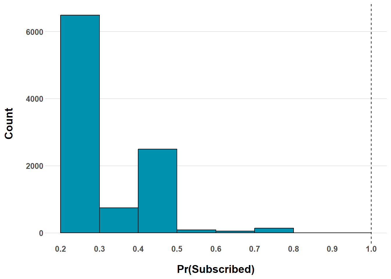
And, as you can see, we are back in the world of possible probabilities!

ggplot(scen4_data, aes(x = p_subscribed, fill = after_stat(x <= 1))) +
  geom_histogram(binwidth = 0.1, boundary = 0, color = "black") +
  scale_x_continuous(breaks = seq(0, 1, by = 0.1)) +
  labs(
    x = "Pr(Subscribed)",
    y = "Count"
  ) +
  scale_fill_manual(
    values = c("TRUE" = colors[2], "FALSE" = colors[6]),
    guide = "none"
  ) +
  geom_vline(xintercept = 1, linetype = "dashed") +
  blog_theme() +
  theme(
    panel.grid.major.x = element_blank(),
    panel.grid.minor.x = element_blank()
  )

Distribution of Probabilities with Varying Effect Sizes and Varying Magnitudes/Signs on Interactions

To avoid redundancy, I am not going to walk through modeling output as the lessons from Scenario 3 are the exact same here in Scenario 4. The main takeaway here is that we only started to observe a distribution of probabilities that was actually possible when we trimmed back on effect sizes and varied the sign and magnitude of the interactive effects. Even under this mostly likely scenario, researchers still have the burden of statistical reporting in light of (hidden) conclusion-altering interactions.

So… on that note, I have some thoughts to share on where you go after you’ve internalized the Piranha Problem.

Test Interactions of Interest

One obvious conclusion is to… start taking interaction effects more seriously and incorporate them as a standard part of your workflow. Even if you don’t plan on reporting out on them, they can serve as a useful pseudo-diagnostic to see how sensitive your average effects are to different contexts. Maybe your stakeholders don’t care if the effect of \(X\) on \(Y\) is moderated by \(M\) because they don’t plan to pull the \(M\) lever anytime soon, but at least you did your due diligence!

Importantly, it’s worth flagging that you’re going to want to be interested in more than just if an interacted effect is statistically different from zero… You’re also going to want to test if the moderation creates statistically different estimates.

For example, the {marginaleffects} syntax below estimates the AMEs for promotion when free_trial = 1 and when free_trial = 0. The hypothesis argument tests to see if these predictions are statistically different from each other (b2 being the estimate for free_trial == 1 and b1 being the estimate for free_trial == 0).

avg_comparisons(scen3_mod_int, variables = "promotion", by = c("free_trial"), hypothesis = "b2 - b1 = 0")

 Hypothesis Estimate Std. Error     z Pr(>|z|)    S 2.5 %  97.5 %
    b2-b1=0   -0.076     0.0226 -3.37   <0.001 10.4 -0.12 -0.0317

Type:  response 

Interactions are Messy…

Of course, if an interaction seems meaningful and your stakeholders are interested, report by all means, but keep in mind that interactions make your model a lot more complicated and that other issues behind the scenes and under the hood are likely to rise up without having the courtesy of giving you a “check engine” flashing light.

Not only do interactions require more statistical power to detect a true effect, but Hainmueller et al. (2019) document other more esoteric issues that arise when employing interaction terms. (Whoever said that good causal inference was remotely simple or easy was lying to you!)

Regularize Your Results

Another key takeaway of the Piranha Problem is that you should generally be very skeptical of large effect sizes, especially if you observe any while exploring the impact of a “new” variable on a well-studied outcome. Don’t ever assume that your data won’t lie to you because, for a variety of reasons, it absolutely will!

In contexts such as these, you can leverage your prior knowledge of skepticism concerning “new” large effects and really make the data prove to you that such a novel, large effect exists. Many folks might be uncomfortable with the use of priors in Bayesian models, for example, but I think the “data-alone” paradigm in frequentist analyses that still dominate much of consulting and academic research would tremendously benefit from a regularization mechanism.

Your prior belief, “variable \(X\) that I’m studying has a small effect on \(Y\)”, could be wrong but it is frankly a much more likely belief than “this new variable \(X\) that has never been evaluated before in this context happens to have a large and stable effect on \(Y\)”. We have some work to do in the realm of reporting out more honest effect sizes and re-framing what the focus of novel research should be. Making the data work harder to prove that new and substantively large effects actually exist is a good step moving forward.

Footnotes

1. One might point out that these values are only possible because I am simulating a linear probability DGP, rather than simulating from a distribution that only allows values between 0 and 1. The choice to use this approach is motivated by the idea to illustrate how thinking through a purely additive model with large effects leads to impossible values. I could, of course, sample from a distribution with the values constrained, but probabilities outside of {0, 1} would just be converted to NA.